Sequences and Series

A sequence is an ordered list generated by a function whose inputs are selected integers. A series is an accumulation formed by adding sequence terms. The distinction between a term $a_n$ and a partial sum $S_n$ is essential because they describe different quantities. Arithmetic patterns arise from repeated addition, while geometric patterns arise from repeated multiplication. This lesson develops formulas by tracing those repeated operations rather than treating them as disconnected rules.

Define a sequence as a function

A sequence is a function whose domain is usually the positive integers or the nonnegative integers. The input is an index, and the output is a term. The notation $a_n$ names the term at index $n$. The subscript is not multiplication. It identifies position in the ordered list.

If a sequence begins $4,7,10,13,\ldots$, then $a_1=4$, $a_2=7$, and $a_3=10$. The ellipsis indicates that the pattern continues, but it does not define the pattern uniquely. Many different rules can begin with the same finite list. A formula or recursion makes the intended continuation explicit. The listed values provide evidence for a rule but are not themselves a complete definition.

Order distinguishes sequences from sets. The sequence $1,2,1$ differs from $1,1,2$ even though both use the same distinct values. Repetition is allowed. The index domain gives every occurrence its place. Applications use this order to represent time steps, positions, iterations, or ranked observations.

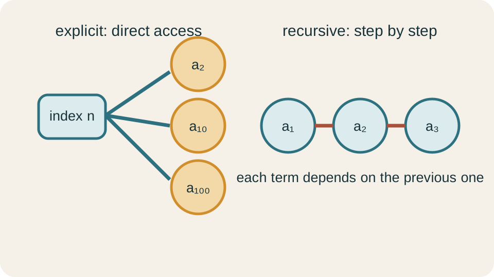
Distinguish explicit and recursive definitions

An explicit rule gives $a_n$ directly from the index $n$. For example, $a_n=4+3(n-1)$ generates $4,7,10,13,\ldots$ when indexing starts at one. Substituting $n=1$ gives the initial term four. Substituting $n=10$ gives the tenth term without computing earlier terms. Explicit formulas support direct access.

A recursive rule defines one or more initial terms and explains how later terms depend on earlier ones. The same sequence can be written $a_1=4$ and $a_n=a_{n-1}+3$ for $n\geq2$. The subscript $n-1$ names the preceding term. Computing $a_{10}$ recursively requires generating the intervening values unless another method is found. Recursions emphasize process and dependence.

Neither representation is universally better. Recursive forms model iterative processes naturally. Explicit forms reveal long-term behavior and allow direct calculation. Some recursions have simple explicit solutions, while others do not. Translating between forms is a central sequence skill.

Track indexing carefully

Indexing may begin at zero, one, or another integer. A formula must match that starting point. If $a_1$ is the first term, then $n-1$ counts the number of steps from index one to index $n$. At $n=1$, zero steps have occurred. This explains why many first-term formulas contain $n-1$.

If indexing begins at zero, the same step count is $n$. A geometric sequence might be written $a_n=a_0r^n$ for $n\geq0$. At $n=0$, the exponent is zero and $a_n=a_0$. Using $n-1$ in this convention would shift every term. The formula should be checked at the starting index.

Changing an index label does not change a sequence if the domain and rule move consistently. The symbols $a_n$ and $a_k$ can describe the same general term under different dummy labels. Fixed references such as $a_1$ are not dummy labels. Index errors often arise from changing one part of notation without changing the others. Substitution at the first two indices is a reliable check.

Recognize arithmetic sequences

An arithmetic sequence has a constant difference between consecutive terms. If that difference is $d$, then $a_n-a_{n-1}=d$. The letter $d$ is a scalar amount added at each step. Positive $d$ produces increasing terms, while negative $d$ produces decreasing terms. Zero $d$ produces a constant sequence.

Starting from $a_1$, one step gives $a_2=a_1+d$. Two steps give $a_3=a_1+2d$. After $n-1$ steps, $a_n=a_1+(n-1)d$. The explicit formula records repeated addition. It is a linear function of index $n$.

For $7,11,15,\ldots$, the common difference is $4$. The twentieth term is $a_{20}=7+(20-1)(4)=83$. The factor nineteen counts the additions from the first term to the twentieth. Using twenty additions would overshoot by one step. Index reasoning explains the calculation.

Model arithmetic change

Arithmetic sequences describe equal additive change per discrete interval. A tank gaining $12.0\,\mathrm{L}$ each minute at recorded whole minutes follows an arithmetic sequence. A salary increasing by a fixed dollar amount each year can also be arithmetic. The common difference carries the same units as the terms. It represents change per index step.

Suppose an account begins with $500\,\mathrm{dollars}$ and receives $75\,\mathrm{dollars}$ at the end of each month without interest. Immediately after month $n$, the balance may be $a_n=500\,\mathrm{dollars}+(75\,\mathrm{\dfrac{dollars}{month}})(n\,\mathrm{months})$. If the initial balance is labeled $a_0$, this formula uses $n$ deposits. If the first recorded term is after one deposit, indexing must reflect that choice. Timeline labels prevent off-by-one errors.

Arithmetic models are inappropriate for constant percentage growth. A fixed percentage creates changes proportional to current amount rather than a fixed difference. The numerical differences then vary. Examining first differences distinguishes additive from multiplicative structure. Context should confirm the pattern rather than relying on a short table alone.

Derive the finite arithmetic sum

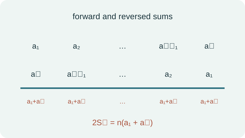
Let $S_n=a_1+a_2+\cdots+a_n$. The capital $S_n$ denotes the sum of the first $n$ terms, not the $n$th term. Write the sum once forward and once backward. Each aligned pair adds to $a_1+a_n$. There are $n$ such pairs across the two written sums.

Therefore $2S_n=n(a_1+a_n)$. Dividing by two gives $S_n=\dfrac{n}{2}(a_1+a_n)$. The horizontal fraction bar groups $n$ over two. The formula equals number of terms times average of first and last term. This average works because arithmetic terms are evenly spaced.

The formula can also be written $S_n=\dfrac{n}{2}[2a_1+(n-1)d]$ after substituting $a_n=a_1+(n-1)d$. Brackets group the entire interior expression. Both forms are equivalent. The first is convenient when the last term is known. The second is convenient when the common difference is known.

Apply an arithmetic sum

Return to the sequence $7,11,15,\ldots$. The fifteenth term is $a_{15}=7+14(4)=63$. The sum of the first fifteen terms is $S_{15}=\dfrac{15}{2}(7+63)=525$. There are fifteen terms, and their average is thirty-five. Multiplication confirms the same total.

A direct listing would be possible but inefficient. The formula uses the pattern’s structure. A magnitude check helps: fifteen terms averaging about thirty-five should total a little over five hundred. The answer $525$ fits that expectation. A result such as $52.5$ would be too small by an order of magnitude.

Units of a series depend on the terms. If each term is a monthly payment in dollars, their sum is total dollars. The index count is dimensionless. Adding terms with incompatible units is invalid. A series is an accumulation of like quantities.

Recognize geometric sequences

A geometric sequence has a constant nonzero ratio between consecutive terms. If the ratio is $r$, then $a_n/a_{n-1}=r$ wherever the denominator is nonzero. Each step multiplies by $r$. Positive $r>1$ gives growth in magnitude for positive starts. A ratio with $|r|<1$ produces decay in magnitude.

Starting from $a_1$, one step gives $a_2=a_1r$. Two steps give $a_3=a_1r^2$. After $n-1$ steps, $a_n=a_1r^{n-1}$. The exponent counts multiplicative steps. This is an exponential function of index.

If $r<0$, term signs alternate. If $r=0$, the standard ratio interpretation becomes delicate after the first zero because division by zero is undefined, though the explicit rule may still generate a sequence. If $r=1$, every term equals $a_1$. Parameter cases affect formulas and behavior. The ratio is part of the model, not merely a calculator input.

Model geometric change

Geometric sequences describe equal multiplicative change per interval. Compound interest, repeated depreciation, population growth under a constant factor, and radioactive decay at equal time steps are common examples. A growth rate $g$ corresponds to factor $1+g$. A decay rate $d$ corresponds to factor $1-d$ when $0<d<1$. Percent language must be converted to a decimal factor.

Equipment initially worth $20{,}000\,\mathrm{dollars}$ retains $85\%$ of its value each year. If $V_0$ is the initial value, then $V_n=(20{,}000\,\mathrm{dollars})(0.85)^n$. The ratio $0.85$ is dimensionless. The exponent $n$ counts yearly retention steps. After one year, the model gives $17{,}000\,\mathrm{dollars}$.

Retaining eighty-five percent is equivalent to depreciating fifteen percent per year in this model. It is not equivalent to subtracting $3{,}000\,\mathrm{dollars}$ every year. The dollar decrease becomes smaller as value falls. Constant difference and constant ratio describe different mechanisms. Tables of differences and ratios can distinguish them.

Derive the finite geometric sum

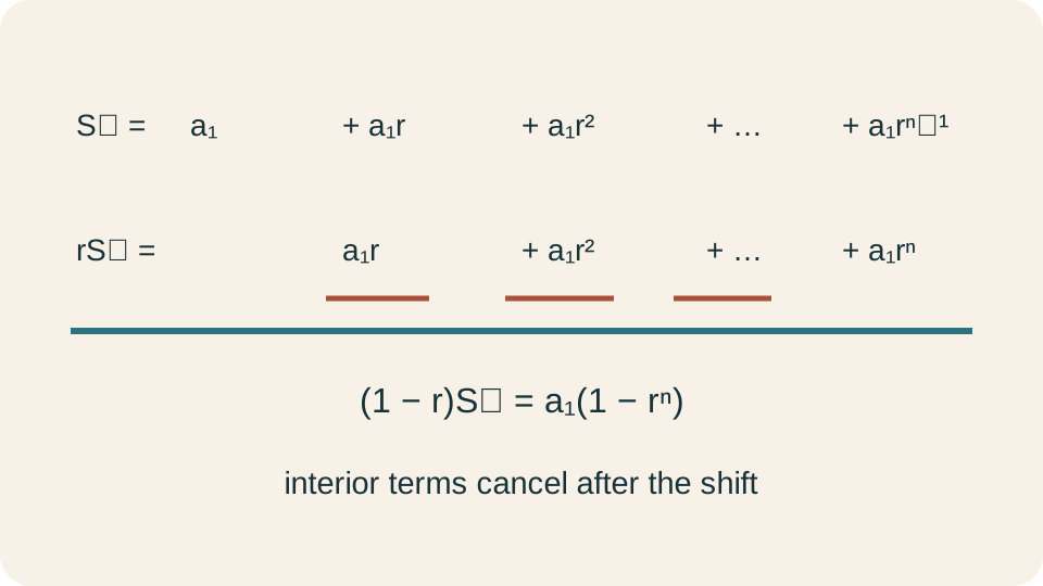
Let $S_n=a_1+a_1r+a_1r^2+\cdots+a_1r^{n-1}$. Multiply by $r$ to obtain $rS_n=a_1r+a_1r^2+\cdots+a_1r^n$. The multiplication shifts every original power one position. Subtract the second equation from the first. All interior terms cancel.

The result is $(1-r)S_n=a_1(1-r^n)$. If $r\neq1$, divide by $1-r$ to get $S_n=a_1\dfrac{1-r^n}{1-r}$. The condition $r\neq1$ is necessary because the denominator would otherwise be zero. When $r=1$, the sum is simply $na_1$. This separate case follows because all $n$ terms are equal.

An equivalent form is $S_n=a_1\dfrac{r^n-1}{r-1}$. Multiplying numerator and denominator by negative one produces it. Either form is valid under the same condition. Choosing a form that keeps intermediate values positive can reduce sign errors. Derivation makes the alternatives easier to recognize.

Apply a finite geometric sum

Suppose a person deposits $100\,\mathrm{dollars}$ at the end of each month into an account earning $0.5\%$ per month. Immediately after the twelfth deposit, the first deposit has earned interest for eleven months. The last deposit has earned none. The balance is $B=(100\,\mathrm{dollars})\sum_{k=0}^{11}(1.005)^k$. The bounds encode twelve deposits and their growth durations.

Using the finite formula gives $B=(100\,\mathrm{dollars})\dfrac{1-(1.005)^{12}}{1-1.005}\approx1{,}233.56\,\mathrm{dollars}$. The denominator and numerator are both negative, so their ratio is positive. Total deposits equal $1{,}200\,\mathrm{dollars}$. The additional $33.56\,\mathrm{dollars}$ is consistent with modest interest. This comparison checks scale.

Deposit timing changes the exponents. Deposits at the beginning of each month would receive one additional month of growth by the same evaluation time. A timeline is more reliable than guessing whether the first exponent is eleven or twelve. Index bounds are part of the financial model. Off-by-one errors have monetary consequences.

Read sigma notation as an instruction

The expression $\sum_{k=1}^{n}a_k$ means $a_1+a_2+\cdots+a_n$. The symbol $k$ is the index of summation. The lower bound gives its first value, and the upper bound gives its last value. The term formula tells what to compute for each index. Sigma notation compresses repeated addition.

To evaluate $\sum_{k=2}^{5}(3k-1)$, substitute $k=2,3,4,5$. The terms are $5,8,11,14$. Their sum is $38$. The number of integer terms is $5-2+1=4$. The plus one includes both endpoints.

The index is a local dummy variable. Replacing $k$ by $j$ does not change the sum if bounds and term formula remain consistent. Thus $\sum_{k=1}^na_k=\sum_{j=1}^na_j$. A free variable outside the sum must not be renamed accidentally. Scope matters in summation notation as it does in functions.

Manipulate finite sums linearly

Summation distributes over addition. The identity is $\sum_{k=1}^n(a_k+b_k)=\sum_{k=1}^na_k+\sum_{k=1}^nb_k$. A constant factor can be moved outside, so $\sum_{k=1}^nca_k=c\sum_{k=1}^na_k$. These rules follow from ordinary distributive and associative properties. They do not depend on a special sequence type.

A constant summed $n$ times gives $\sum_{k=1}^nc=nc$. The index does not appear in the term, but the bounds still control repetition count. For example, $\sum_{k=3}^{7}4=5(4)=20$. There are five terms, not seven. Count comes from upper minus lower plus one.

Bounds can be split at an interior index. For $m<n$, $\sum_{k=1}^na_k=\sum_{k=1}^ma_k+\sum_{k=m+1}^na_k$. No term may be duplicated or omitted. This property supports partial accumulation and algorithms. Drawing the index list verifies the split.

Distinguish terms from partial sums

Given sequence $a_1,a_2,\ldots$, define the partial sum $S_n=\sum_{k=1}^na_k$. The sequence $(S_n)$ is a new sequence. Its terms record accumulated totals. It differs from the original term sequence $(a_n)$. Confusing them leads to incorrect convergence claims.

The relation between them is $S_n-S_{n-1}=a_n$ for $n\geq2$. The newest term is the increment in accumulated sum. Conversely, $S_n=S_{n-1}+a_n$. This recursion links local contribution with cumulative total. It is a discrete analogue of derivative and integral relationships.

For $a_n=1$ for every $n$, terms approach one while partial sums grow as $S_n=n$. For $a_n=\dfrac{1}{2^n}$, terms approach zero and partial sums approach a finite limit. Term behavior and sum behavior answer different questions. A series converges only when its partial-sum sequence converges. Inspecting $a_n$ alone cannot establish the final accumulated value.

Define an infinite series through a limit

An infinite series is not completed by literally adding a final term. It is defined as the limit of partial sums. The notation $\sum_{k=1}^{\infty}a_k=\lim_{n\to\infty}\sum_{k=1}^na_k$ expresses this definition. The arrow means that the number of included terms grows without bound. If partial sums approach a finite value, the series converges.

If partial sums do not approach a finite value, the series diverges. They may grow without bound, oscillate, or behave irregularly. Divergence is not always the same as approaching infinity. The definition asks for one finite limiting sum. Partial sums provide the evidence.

A necessary condition for convergence is $a_n\to0$. If terms do not approach zero, adding further terms cannot settle the partial sums. The condition is not sufficient. The harmonic series has $a_n=1/n\to0$ but diverges. Term tests can disprove convergence without always proving it.

Derive the infinite geometric sum

For a geometric series beginning at index zero, the partial sum is $S_n=a\dfrac{1-r^{n+1}}{1-r}$ when it includes terms through $r^n$. If $|r|<1$, then $r^{n+1}\to0$. The partial sums approach $\dfrac{a}{1-r}$. Therefore $\sum_{k=0}^{\infty}ar^k=\dfrac{a}{1-r}$ for $|r|<1$. The limit converts a sequence of finite sums into the defined infinite-series value.

The absolute-value condition is part of the formula. If $r=1$, partial sums grow by $a$. If $r=-1$ with nonzero $a$, partial sums oscillate. If $|r|>1$, term magnitudes grow. None of these cases produces a finite limiting sum.

For $\sum_{k=0}^{\infty}5\left(-\dfrac{1}{3}\right)^k$, the ratio magnitude is $\dfrac{1}{3}<1$. The sum is $\dfrac{5}{1-(-1/3)}=\dfrac{15}{4}$. Alternating signs make partial sums approach the limit from opposite sides. The finite value follows from the partial-sum limit, not from stopping the series. Every additional term changes the partial sum by a smaller amount.

Interpret convergence visually

Plotting $a_n$ against index shows term behavior. Plotting $S_n$ against index shows accumulated behavior. A convergent series has partial-sum points approaching a horizontal level. Its term points must approach zero. The two graphs should not be confused.

For a positive geometric ratio below one, partial sums approach the limit from one side. For a negative ratio with magnitude below one, they oscillate with decreasing amplitude around the limit. A ratio near one produces slow convergence. The formula and graph describe the same rate behavior. Visual patterns support limit reasoning.

Finite decimal representations illustrate geometric convergence. The repeating decimal $0.333\ldots$ equals $\dfrac{3}{10}+\dfrac{3}{100}+\dfrac{3}{1000}+\cdots$. This geometric series has first term $3/10$ and ratio $1/10$. Its sum is $\dfrac{3/10}{1-1/10}=\dfrac{1}{3}$. Infinite representation can equal a finite number through a limit.

Diagnose common sequence errors

One mistake is confusing $a_n$ with $S_n$. The first is a term, and the second is an accumulated sum. Another is using $n$ instead of $n-1$ when $a_1$ is the initial term. Substituting the starting index reveals the shift. Index checks are faster than repairing a full calculation.

Another error is classifying constant percentage growth as arithmetic. Arithmetic sequences have constant differences. Geometric sequences have constant ratios. A short data table can sometimes mimic both approximately, so context matters. Computing several differences and ratios provides evidence.

Infinite-series errors include applying the geometric sum when $|r|\geq1$ or assuming $a_n\to0$ proves convergence. The convergence condition belongs with the formula. A finite sum always exists, but an infinite series requires a limiting argument. Writing the partial sum first keeps this distinction visible. A formula without its convergence condition is incomplete.

Practice a complete sequence routine

First state the index domain and initial term. Second determine whether change is additive, multiplicative, recursive, or another pattern. Third write a rule and test it at the first two indices. Fourth distinguish whether the question asks for one term or an accumulated sum. Fifth check units, size, and index count.

For $a_n=3\left(\dfrac{1}{2}\right)^{n-1}$ with $n\geq1$, the first five terms are $3,\dfrac{3}{2},\dfrac{3}{4},\dfrac{3}{8},\dfrac{3}{16}$. The ratio is one-half. The fifth exponent is four because four multiplications occur after the first term. Each term is positive and half the preceding one. The behavior matches the formula.

For $\sum_{k=1}^{4}(2k+1)$, the terms are $3,5,7,9$. Their sum is $24$. The same list is arithmetic with first term three and last term nine. The arithmetic formula gives $\dfrac{4}{2}(3+9)=24$. Two methods provide a check.

Consolidate sequence and series reasoning

A sequence is a function on an ordered integer domain. Explicit rules provide direct terms, while recursive rules describe generation. Arithmetic patterns repeat addition, and geometric patterns repeat multiplication. Their exponents and coefficients count steps from a declared starting index. Indexing is part of the model.

A series adds sequence terms. Finite arithmetic sums follow from equal pairing, while finite geometric sums follow from shifting and cancellation. Sigma notation specifies index, bounds, and term formula compactly. Partial sums form a separate sequence of accumulated values. Infinite series are defined through limits of those partial sums.

Reliable work distinguishes terms from sums and checks the first index. It carries units through applications and uses timelines for repeated deposits or changes. It states convergence conditions alongside infinite formulas. Deriving structure reduces dependence on memorization. Sequences describe ordered change, and series describe what that change accumulates.