Infinite Series and Convergence

An infinite series is not an instruction to finish infinitely many additions. It is a limit question about a sequence of finite totals. This definition separates the terms being added from the partial sums whose behavior determines convergence. Once that distinction is secure, convergence tests become reasoned comparisons rather than names attached to visual patterns. This lesson builds a selection strategy, verifies every test’s hypotheses, and connects convergence to usable approximation error.

Learning objectives and the two-sequence distinction

By the end of this lesson, you will define an infinite series through its partial sums. You will analyze geometric, telescoping, positive-term, and alternating series. You will choose among divergence, comparison, integral, ratio, and root tests based on structure. You will distinguish absolute convergence from conditional convergence. You will also use remainder estimates to decide how many terms an approximation needs.

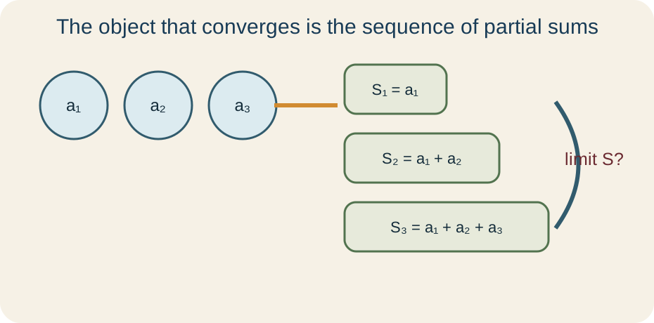
Every series involves two related sequences. The term sequence $\{a_n\}$ lists the individual quantities being added. The partial-sum sequence $\{S_N\}$ lists accumulated totals, where $S_N=\sum_{n=1}^{N}a_n$. The index $n$ identifies a term, while the capital index $N$ identifies the last included term. Convergence concerns the behavior of $S_N$, not merely the behavior of $a_n$.

This distinction prevents the most common conceptual error. The condition $a_n\to0$ says that successive additions become small, but small additions can accumulate without settling. Convergence requires the accumulated totals to approach one finite number. The diagram below shows terms feeding partial sums and partial sums approaching a possible limit. Every convergence test ultimately supplies evidence about that final arrow.

Define convergence through partial sums

For a sequence of terms $a_n$, define $S_N=\sum_{n=1}^{N}a_n$. The sigma symbol $\sum$ means add the expression to its right while the index runs from the lower bound to the upper bound. Thus $S_3=a_1+a_2+a_3$. The infinite series $\sum_{n=1}^{\infty}a_n$ converges to $S$ when $\lim_{N\to\infty}S_N=S$. If no finite limit exists, the series diverges.

The definition does not require an infinite computation. For each finite $N$, calculate or reason about a finite partial sum. Then analyze what happens as $N$ grows without bound. The symbol $\infty$ is not a number substituted for $N$; it describes unbounded growth of the index. A convergent series assigns a finite limiting value to that process.

Finite changes at the beginning do not alter whether a series converges. Adding or removing ten terms changes later partial sums by one constant amount. A convergent tail therefore remains convergent, and a divergent tail remains divergent. The starting index can affect the numerical sum but not the convergence classification. This fact allows tests to focus on sufficiently large $n$, where structure is often simpler.

Use the term test correctly

If $\sum a_n$ converges, then necessarily $a_n\to0$. To see why, note that $a_N=S_N-S_{N-1}$. If both partial sums approach the same limit $S$, their difference approaches zero. Therefore a nonzero term limit, an infinite term limit, or a nonexistent term limit proves divergence. This result is commonly called the divergence test or nth-term test.

The converse is false. The harmonic series $\sum_{n=1}^{\infty}\frac{1}{n}$ has terms approaching zero but diverges. Group terms after the first into blocks whose sizes double. Each block contributes at least $\frac{1}{2}$ because it contains enough terms, each no smaller than the block’s final term. Infinitely many contributions of at least one half force partial sums upward without bound.

Use the term test as an early filter. If the term limit is not zero, stop and conclude divergence. If the term limit is zero, write that the test is inconclusive rather than claiming convergence. Then inspect the series for another structure. Passing a necessary condition is not the same as satisfying a sufficient condition.

Analyze geometric and telescoping series

A geometric series has the form $\sum_{n=0}^{\infty}ar^n$, where $a$ is the first term and $r$ is the common ratio. Its finite partial sum is $S_N=a\frac{1-r^{N+1}}{1-r}$ when $r\ne1$. The horizontal fraction bar groups the entire numerator over $1-r$. If $|r|<1$, then $r^{N+1}\to0$. Consequently the infinite sum is $\frac{a}{1-r}$.

If $|r|\ge1$, the terms generally do not approach zero, so a nontrivial geometric series diverges. For $r=-\frac{1}{2}$, signs alternate but magnitudes shrink, so convergence still occurs. For $r=-2$, magnitudes grow and the term test proves divergence. The absolute value condition captures both positive and negative ratios. Always identify the first term for the actual starting index rather than assuming it equals the coefficient shown.

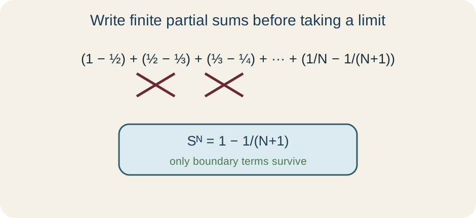
A telescoping series cancels many terms across consecutive partial sums. For example, $\sum_{n=1}^{\infty}\left(\frac{1}{n}-\frac{1}{n+1}\right)$ has partial sum $S_N=1-\frac{1}{N+1}$. Writing several terms makes the cancellation visible. Taking the limit gives a sum of one. Telescoping is a partial-sum computation, so state the surviving boundary terms before taking a limit.

Compare positive-term series

Direct comparison transfers convergence through inequalities. If $0\le a_n\le b_n$ for sufficiently large $n$ and $\sum b_n$ converges, then $\sum a_n$ converges. If $0\le b_n\le a_n$ and $\sum b_n$ diverges, then $\sum a_n$ diverges. A smaller nonnegative series below a convergent ceiling must converge. A larger nonnegative series above a divergent floor must diverge.

Benchmark series guide the comparison. The $p$-series $\sum_{n=1}^{\infty}\frac{1}{n^p}$ converges exactly when $p>1$. For $n\ge1$, $0\le\frac{1}{n^2+4}\le\frac{1}{n^2}$. Since the comparison series has $p=2>1$, it converges. Direct comparison therefore proves that $\sum\frac{1}{n^2+4}$ converges.

Inequality direction must match the desired conclusion. Showing a series is smaller than a divergent series proves nothing, because a smaller series might converge or diverge. Showing a series is larger than a convergent series is equally inconclusive. Denominator comparisons often reverse intuition: a larger positive denominator creates a smaller fraction. State nonnegativity and the relevant index range before applying the theorem.

Use limit comparison for dominant behavior

The limit comparison test handles positive terms whose inequality is awkward but whose long-run scale is recognizable. If $a_n>0$, $b_n>0$, and $\lim_{n\to\infty}\frac{a_n}{b_n}=L$ with $0<L<\infty$, then the two series share a convergence classification. A finite positive ratio means their terms are asymptotically comparable. Neither sequence eventually overwhelms the other by an unbounded factor. Choose $b_n$ from a known benchmark family.

For $a_n=\frac{3n+1}{n^3-4}$, dominant powers suggest comparison with $b_n=\frac{1}{n^2}$. The ratio is $\frac{a_n}{b_n}=\frac{3n^3+n^2}{n^3-4}$. Dividing numerator and denominator by $n^3$ gives a limit of three. Since $3$ is finite and positive and $\sum\frac{1}{n^2}$ converges, the original series converges. The calculation makes the phrase “behaves like $\frac{3}{n^2}$” precise.

Limit comparison may fail to decide when $L=0$ or $L=\infty$, although one-sided conclusions are sometimes available. In an introductory course, choose a more comparable benchmark or return to direct comparison. Also verify eventual positivity because sign changes require different tools. Dominant powers are a selection heuristic, not the theorem itself. The limit and benchmark conclusion together form the proof.

Apply the integral test and estimate tails

The integral test applies when $a_n=f(n)$ for a function $f$ that is positive, continuous, and decreasing for all sufficiently large inputs. Under those hypotheses, $\sum_{n=N}^{\infty}a_n$ and $\int_N^{\infty}f(x)\,dx$ either both converge or both diverge. The test connects rectangular sums with area under a curve. Positivity prevents cancellation from hiding accumulated size. Decrease lets rectangles bound the tail consistently.

For $f(x)=\frac{1}{x^p}$, the improper integral $\int_1^{\infty}x^{-p}\,dx$ converges exactly when $p>1$. This proves the $p$-series criterion. At $p=1$, the antiderivative is $\ln x$, which grows without bound. For $p<1$, the power antiderivative also grows without bound. The boundary at one is therefore a consequence of improper-integral behavior.

The same geometry gives remainder bounds. If $R_N=S-S_N$ is the uncomputed tail, then $\int_{N+1}^{\infty}f(x)\,dx\le R_N\le\int_N^{\infty}f(x)\,dx$. The symbol $R_N$ denotes error after keeping terms through index $N$. These inequalities can choose $N$ before doing extensive arithmetic. A convergence proof says a limit exists, while an error bound says how close a finite approximation is.

Use ratio and root tests for exponential tendency

The ratio test examines $L=\lim_{n\to\infty}\left|\frac{a_{n+1}}{a_n}\right|$. If $L<1$, the series converges absolutely. If $L>1$ or $L$ is infinite, the terms fail to shrink sufficiently and the series diverges. If $L=1$, the test is inconclusive. The absolute value makes the test analyze magnitude regardless of sign.

Factorials and exponentials often simplify under successive-term ratios. For $a_n=\frac{3^n}{n!}$, the factorial notation means $n!=n(n-1)\cdots2\cdot1$. The ratio simplifies to $\frac{3}{n+1}$ because most factors cancel. Its limit is zero, which is less than one. Therefore $\sum\frac{3^n}{n!}$ converges absolutely.

The root test uses $L=\lim_{n\to\infty}\sqrt[n]{|a_n|}$ with the same three conclusions. It is especially useful when the entire term is raised to the $n$th power. Both tests compare long-run magnitude with a geometric series. They often return $L=1$ for rational-power terms such as $1/n^p$. In that case, use a $p$-series, comparison, or integral test instead.

Analyze alternating and signed series

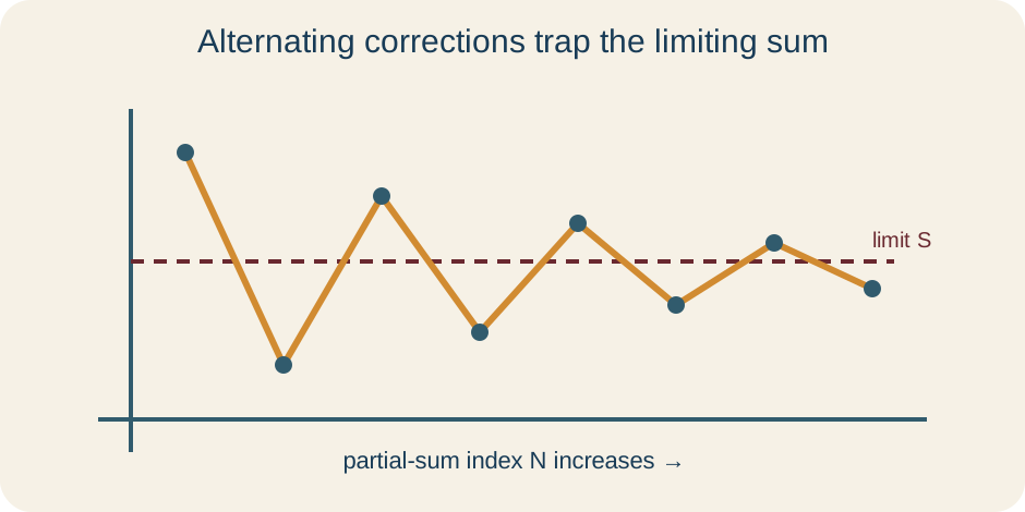
An alternating series changes sign in a regular pattern, often written $\sum(-1)^{n}b_n$ or $\sum(-1)^{n+1}b_n$ with $b_n\ge0$. The alternating-series test requires $b_n\to0$ and eventual nonincrease of $b_n$. Under those hypotheses, positive and negative corrections trap the partial sums around one limit. The decreasing magnitude prevents later corrections from undoing control gained earlier. Both hypotheses must be stated.

For the alternating harmonic series $\sum_{n=1}^{\infty}\frac{(-1)^{n+1}}{n}$, the magnitudes $1/n$ decrease to zero. Therefore the alternating-series test proves convergence. However, the absolute series is the divergent harmonic series. The original series converges conditionally rather than absolutely. Conditional convergence depends essentially on cancellation.

If $\sum|a_n|$ converges, then $\sum a_n$ converges absolutely. Absolute convergence is stronger and remains stable under rearrangement. A conditionally convergent series can change sum or diverge when terms are rearranged, a fact known as the Riemann rearrangement phenomenon. This sensitivity shows why “positive and negative terms cancel” is not a complete justification. One must classify the magnitude series separately.

Quantify approximation error

For an alternating series satisfying its test, the error after $N$ terms obeys $|R_N|\le b_{N+1}$. The vertical bars mean error magnitude, so the bound ignores whether the approximation is above or below the limit. The next omitted term controls the maximum error. This is the alternating-series estimation theorem. It converts qualitative convergence into a stopping rule.

Suppose $\sum_{n=1}^{\infty}\frac{(-1)^{n+1}}{n^3}$ is approximated with error below $0.001$. The next-term bound requires $\frac{1}{(N+1)^3}<0.001$. Since $0.001=\frac{1}{1000}$, it is enough that $(N+1)^3>1000$. Thus $N+1>10$, so choosing $N=10$ gives a bound at most $\frac{1}{1331}$, which is below the target. Ten retained terms therefore guarantee the requested accuracy.

Different tests supply different error information. A geometric tail can often be summed exactly as another geometric series. The integral test provides upper and lower bounds for positive decreasing tails. Ratio and root tests usually classify convergence without immediately giving a classroom-ready sharp bound. Always match the error theorem to hypotheses already verified. Report both the approximation and its guaranteed tolerance.

Choose a test strategically

Begin with the term limit because it can prove divergence immediately. Then look for exact structure such as geometric form or telescoping cancellation. For nonnegative rational expressions, compare dominant powers with a $p$-series. For terms involving factorials or repeated exponentials, try the ratio test. For an $n$th power of a complicated expression, consider the root test.

For alternating signs, first test absolute convergence using the magnitude series. If that fails or is known to diverge, check the alternating-series hypotheses. An integral test is natural when the term comes from a positive continuous decreasing function with a manageable antiderivative. No ranking makes one test universally better. Good selection comes from matching algebraic structure to a theorem’s hypotheses.

An inconclusive test is not a failed solution. It is information that sends you to a different tool. The ratio test returning one does not imply divergence, because both the convergent series $\sum1/n^2$ and divergent series $\sum1/n$ produce that result. Record what was learned and change methods. The decision map below summarizes this reasoning without replacing proof.

Guided practice and synthesis

Classify $\sum_{n=1}^{\infty}3\left(\frac{1}{4}\right)^{n-1}$. It is geometric with first term three and ratio one fourth. Since the ratio magnitude is below one, it converges. Its sum is $\frac{3}{1-\frac{1}{4}}=4$. The horizontal fraction bars show complete numerator-to-denominator division.

Classify $\sum_{n=1}^{\infty}\frac{(-1)^{n+1}}{n^2}$. The absolute-value series is the $p$-series $\sum\frac{1}{n^2}$ with $p=2>1$. Therefore the original series converges absolutely. The alternating-series test would prove convergence but would not provide the stronger classification by itself. Test absolute convergence first whenever it is accessible.

For independent synthesis, analyze $\sum_{n=2}^{\infty}\frac{n+2}{n^3-1}$. Begin with the term limit, choose a benchmark from dominant powers, and verify eventual positivity. Compute the required comparison limit and state the benchmark’s classification. Then explain why the ratio test is likely to return an inconclusive limit. Finish by distinguishing the term sequence from the partial-sum sequence in this example.

Connection forward

Convergence is a statement about limits of finite partial sums. Exact families, comparison theorems, integral geometry, and exponential-tendency tests provide different routes to that statement. Absolute convergence controls magnitude before cancellation, while conditional convergence depends on sign arrangement. Error estimates determine whether a finite computation meets a stated tolerance. These ideas make infinite processes mathematically usable.

The most rigorous solution names the chosen theorem and checks every hypothesis. It explains why a benchmark is comparable, why a function decreases, or why a magnitude sequence tends to zero. It treats an inconclusive result honestly and chooses another test. It also distinguishes proving convergence from calculating the sum. Most convergence tests settle existence without revealing a closed-form value.

Taylor and Maclaurin series use infinite sums to represent functions. Their usefulness depends on the interval of convergence and on control of truncation error. Power series also introduce a variable into the terms, so convergence may change with the input. The foundation remains the same partial-sum limit developed here. A function representation is trustworthy only where that limit and its error have been justified.