Taylor and Maclaurin Series

A Taylor polynomial replaces a complicated function with a polynomial that matches its local behavior at a chosen center. It matches the function value, slope, concavity, and increasingly higher derivative information as its degree grows. A Taylor series asks whether this matching process can continue indefinitely and whether the resulting infinite series actually equals the original function. Those are related but distinct questions. This lesson develops the construction, the convergence logic, and the error controls needed to use the method responsibly.

Learning objectives

By the end of the lesson, you should be able to derive the coefficient formula for a Taylor polynomial. You should construct Taylor and Maclaurin polynomials directly from derivatives. You should interpret every symbol in summation notation and explain why factorials appear. You should recognize and transform several foundational Maclaurin series. Every formula should be connected to the derivative-matching goal that produced it.

You will distinguish a finite Taylor polynomial, a formal Taylor series, a convergent power series, and a proven function representation. You will determine radii and intervals of convergence and test endpoints separately. You will calculate approximations and use Lagrange or alternating-series error bounds. You will also choose a polynomial degree from a requested tolerance. These skills turn approximation into a quantified argument rather than an unsupported decimal estimate.

Keep three questions separate throughout the lesson. What polynomial matches the first $n$ derivatives, where does the infinite power series converge, and where does its sum equal the function? A successful coefficient calculation answers only the first question. A ratio test often answers the second. A remainder tending to zero connects the series back to the function and answers the third.

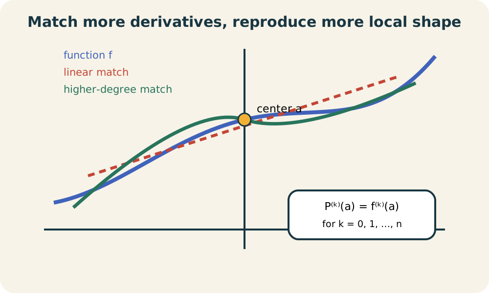
Begin with local matching

Suppose a polynomial is centered at $x=a$. Write it as $P_n(x)=c_0+c_1(x-a)+c_2(x-a)^2+\cdots+c_n(x-a)^n$. The subscript $n$ indicates degree, and the coefficients $c_0$ through $c_n$ are initially unknown. Centered powers are used because most terms vanish when $x=a$. That vanishing isolates coefficients one derivative at a time.

Matching function value requires $P_n(a)=f(a)$. Substitution makes every positive power of $a-a$ equal zero. Only $c_0$ remains, so $c_0=f(a)$. Matching first derivatives requires $P_n'(a)=f'(a)$. Differentiation and evaluation leave $c_1=f'(a)$.

Matching the second derivative gives $P_n''(a)=2!c_2=f''(a)$. The factorial $2!=2\cdot1$ counts the derivative multipliers accumulated from $(x-a)^2$. More generally, differentiating $(x-a)^k$ exactly $k$ times produces $k!$. Evaluating at the center eliminates every term not aligned with that derivative order. Therefore $c_k=\frac{f^{(k)}(a)}{k!}$.

The Taylor polynomial formula

Substituting the derived coefficients gives $P_n(x)=\sum_{k=0}^{n}\frac{f^{(k)}(a)}{k!}(x-a)^k$. The summation index $k$ begins at zero and ends at $n$. The notation $f^{(k)}(a)$ means the $k$th derivative evaluated at the center. By convention, $f^{(0)}=f$ and $0!=1$. The first summand is therefore $f(a)$.

Writing the first few terms makes the structure visible. The polynomial is $f(a)+f'(a)(x-a)+\frac{f''(a)}{2!}(x-a)^2+\frac{f'''(a)}{3!}(x-a)^3+\cdots$. The constant term matches value. The linear term matches slope, and the quadratic term matches concavity. Higher powers encode progressively finer local derivative behavior.

When the center is $a=0$, the construction is called a Maclaurin polynomial. Its formula is $P_n(x)=\sum_{k=0}^{n}\frac{f^{(k)}(0)}{k!}x^k$. Maclaurin is not a different method. It is the Taylor construction at the special center zero. A different center may approximate a target point more efficiently when it lies closer to that point.

Why factorials cannot be omitted

The factorial denominator reverses the multipliers created by repeated differentiation. Without it, the $k$th derivative at the center would be $k!$ times too large. For example, the second derivative of $c_2(x-a)^2$ at $a$ is $2c_2$. Choosing $c_2=\frac{f''(a)}{2}$ makes the match exact. The same logic continues for every degree.

Factorial growth also influences approximation behavior. The value $k!$ grows as $1\cdot2\cdot3\cdots k$. For many smooth functions, division by factorial makes higher-order terms small near the center. This suppression helps series such as the exponential converge for every real input. It does not by itself prove every Taylor series represents its function.

Dimensional reasoning can provide another check in applied settings. If $x$ carries units, the coefficient of $(x-a)^k$ must carry reciprocal powers so each term has the units of $f$. The derivative $f^{(k)}$ naturally has those reciprocal units. Dividing by the dimensionless factorial does not change them. Adding terms with incompatible units would expose an invalid construction.

Building the exponential series

For $f(x)=e^x$, every derivative is $e^x$. At the Maclaurin center, every derivative value is $e^0=1$. Therefore the degree-$n$ polynomial is $P_n(x)=\sum_{k=0}^{n}\frac{x^k}{k!}$. Letting the degree increase suggests $e^x=\sum_{k=0}^{\infty}\frac{x^k}{k!}$. The infinite upper limit means partial sums continue without a final term.

The first terms are $1+x+\frac{x^2}{2!}+\frac{x^3}{3!}+\cdots$. At $x=0$, the constant term gives the correct value one. Differentiating term by term reproduces the same series, matching the defining derivative property of $e^x$. This structural consistency explains why the series is natural. A remainder argument will later justify equality.

At $x=0.5$, the degree-four approximation is $1+0.5+\frac{0.5^2}{2!}+\frac{0.5^3}{3!}+\frac{0.5^4}{4!}=1.6484375$. Every term is dimensionless because the pure exponential’s argument must be dimensionless. Each added term refines the local derivative match. The approximation is close to the true value, but closeness should not be asserted from appearance alone. An error bound turns that observation into a guarantee.

Sine and cosine from derivative cycles

The derivatives of sine cycle through $\sin x$, $\cos x$, $-\sin x$, and $-\cos x$. At zero, their values cycle through $0,1,0,-1$. Even-power coefficients vanish, leaving $\sin x=\sum_{k=0}^{\infty}\frac{(-1)^kx^{2k+1}}{(2k+1)!}$. The exponent $2k+1$ generates odd powers. The factor $(-1)^k$ alternates signs.

Cosine derivatives follow the same cycle but begin with cosine. At zero, values cycle through $1,0,-1,0$. Odd-power coefficients vanish, leaving $\cos x=\sum_{k=0}^{\infty}\frac{(-1)^kx^{2k}}{(2k)!}$. The exponent $2k$ generates even powers. This even-only structure agrees with cosine’s symmetry.

These formulas assume angles in radians. The familiar derivative identities for sine and cosine take their simple form only in radian measure. A degree-five sine polynomial is $x-\frac{x^3}{3!}+\frac{x^5}{5!}$. A degree-four cosine polynomial is $1-\frac{x^2}{2!}+\frac{x^4}{4!}$. Their parity and alternating signs can be reconstructed from derivative cycles rather than memorized in isolation.

The geometric series as a generator

The geometric identity is $\frac{1}{1-x}=\sum_{k=0}^{\infty}x^k$ for $|x|<1$. Its partial sums satisfy $1+x+\cdots+x^n=\frac{1-x^{n+1}}{1-x}$. When $|x|<1$, the remainder term $x^{n+1}$ approaches zero. This proves the infinite identity in that interval. When $|x|\ge1$, the terms fail to approach zero in the required way for this series.

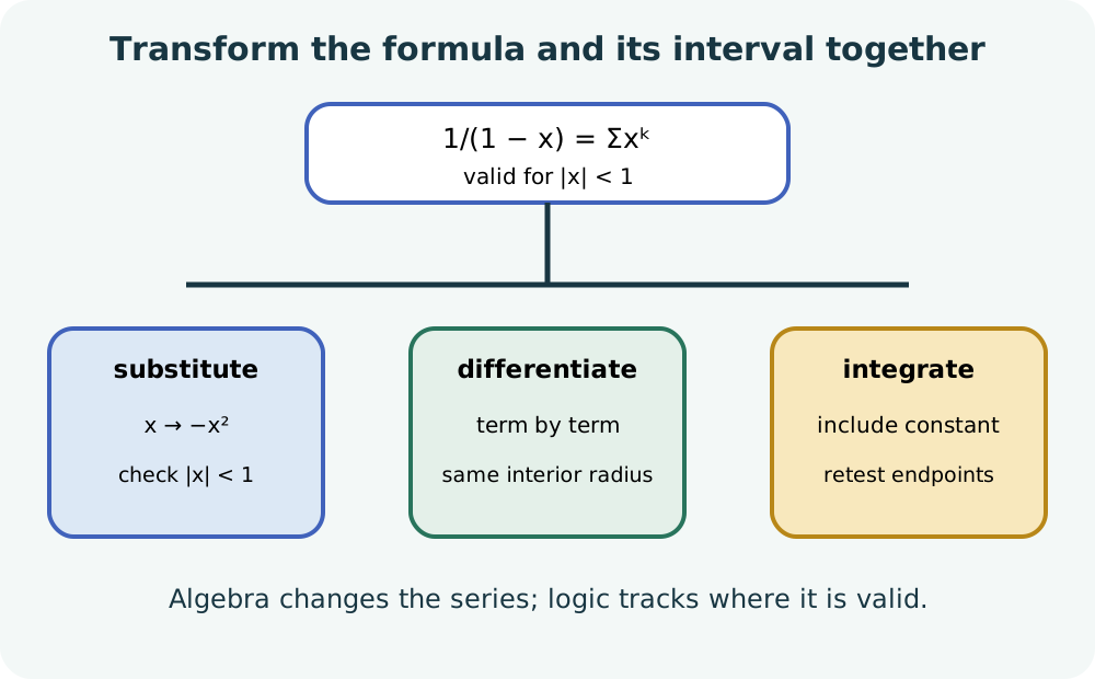
Many power series can be generated by substituting, differentiating, or integrating this identity. Replacing $x$ with $-x$ gives $\frac{1}{1+x}=\sum_{k=0}^{\infty}(-1)^kx^k$ for $|x|<1$. Replacing $x$ with $-x^2$ gives $\frac{1}{1+x^2}=\sum_{k=0}^{\infty}(-1)^kx^{2k}$ for $|x|<1$. The new powers and signs follow directly from the substituted expression. The convergence condition must be transformed with the algebra.

Integrating the last series from zero to $x$ yields $\arctan x=\sum_{k=0}^{\infty}\frac{(-1)^kx^{2k+1}}{2k+1}$ within the justified interior interval. The integration constant is fixed because both sides equal zero at $x=0$. Each denominator $2k+1$ comes from integrating the corresponding power. Endpoints $x=1$ and $x=-1$ require separate convergence tests. Formal manipulation alone does not settle them.

Polynomial, series, and representation

A Taylor polynomial has finitely many terms and is defined wherever ordinary polynomial arithmetic is defined. It approximates a function locally by matching a finite number of derivatives. A Taylor series is the infinite formal expression $\sum_{k=0}^{\infty}\frac{f^{(k)}(a)}{k!}(x-a)^k$. That expression may converge for some values and diverge for others. Convergence produces a sum function.

Even when the series converges, its sum need not equal the original function everywhere. Equality requires the remainder $R_n(x)=f(x)-P_n(x)$ to approach zero as $n$ approaches infinity. Derivative matching at one point is local information. An infinitely differentiable function can have all derivatives zero at a point while remaining nonzero elsewhere. Smoothness alone is not enough.

A function equal to its Taylor series near a point is called analytic there. Familiar elementary functions such as exponential, sine, and cosine are analytic throughout their real domains. Other functions have more limited representation intervals because of nearby singular behavior. The distinction between smooth and analytic is mathematically significant. It prevents “infinitely many matching derivatives” from being mistaken for an automatic global identity.

Radius and interval of convergence

A power series centered at $a$ typically converges for $|x-a|<R$ and diverges for $|x-a|>R$. The nonnegative number $R$ is the radius of convergence. The interval from $a-R$ to $a+R$ is the interior convergence interval. If $R=\infty$, the series converges for every real $x$. If $R=0$, it converges only at the center.

The ratio test often determines $R$. For terms $u_k$, examine $\lim_{k\to\infty}\left|\frac{u_{k+1}}{u_k}\right|$. Requiring that limit to be less than one produces an inequality involving $|x-a|$. Solve the inequality for the interior interval. The ratio test commonly becomes inconclusive when the limit equals one at endpoints.

Each finite endpoint must be tested as its own numerical series. One endpoint may converge while the other diverges. An endpoint can also converge conditionally rather than absolutely. Interior conclusions do not automatically include boundary points. The final answer should use interval notation after both tests are complete.

Convergence example with endpoint tests

Consider $\sum_{k=1}^{\infty}\frac{(x-2)^k}{k3^k}$. The ratio of absolute terms approaches $\frac{|x-2|}{3}$. Requiring this value below one gives $|x-2|<3$. The preliminary interval is $-1<x<5$. The radius is $R=3$ and the center is $a=2$.

At $x=5$, the series becomes $\sum_{k=1}^{\infty}\frac{1}{k}$, which diverges. At $x=-1$, it becomes $\sum_{k=1}^{\infty}\frac{(-1)^k}{k}$, which converges by the alternating-series test. The alternating endpoint is conditional because the corresponding absolute series diverges. The left endpoint is included and the right endpoint is excluded. The convergence interval is $[-1,5)$.

The example shows why “radius three” is not the complete answer. Radius describes the symmetric interior around the center. Endpoint behavior can break symmetry. Absolute convergence holds in the open interior, while the included endpoint is conditional in this example. A full solution reports radius, interval, and endpoint reasoning.

The Lagrange remainder

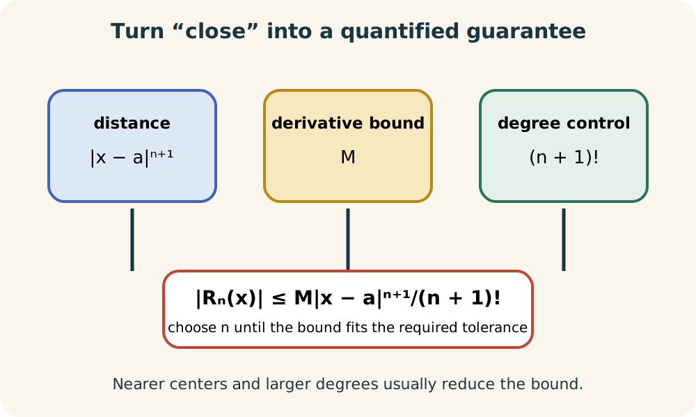
The Lagrange form of the remainder is $R_n(x)=\frac{f^{(n+1)}(c)}{(n+1)!}(x-a)^{n+1}$ for some $c$ between $a$ and $x$, under suitable differentiability conditions. The unknown location $c$ depends on $x$ and the approximation. We usually do not calculate it directly. Instead, we bound the derivative over the entire interval between center and target. This converts an existence statement into a usable inequality.

If $|f^{(n+1)}(t)|\le M$ throughout that interval, then $|R_n(x)|\le\frac{M|x-a|^{n+1}}{(n+1)!}$. The constant $M$ bounds the next derivative. Distance from the center appears through $|x-a|^{n+1}$. Degree appears through both the exponent and factorial. A smaller bound guarantees greater accuracy.

The bound need not equal the actual error. It is a worst-case guarantee based on available derivative information. A loose $M$ can produce a conservative estimate. The theorem’s value lies in certifying that error cannot exceed the bound. It supports decisions about how many terms are sufficient.

Controlled cosine approximation

Use $P_4(x)=1-\frac{x^2}{2!}+\frac{x^4}{4!}$ to approximate $\cos(0.20)$. Substitution gives $1-\frac{(0.20)^2}{2}+\frac{(0.20)^4}{24}$. Evaluating yields approximately $0.9800667$. The center is zero and the target is only $0.20$ radians away. This proximity supports good local accuracy.

The degree-four Lagrange remainder uses the fifth derivative. Every derivative of cosine or sine has magnitude at most one, so choose $M=1$. The bound is $|R_4(0.20)|\le\frac{(0.20)^5}{5!}=2.67\times10^{-6}$. Therefore the true cosine value lies within that distance of the polynomial estimate. The bound is stated before rounding the reported answer.

An even sharper observation uses the cosine series structure. The degree-four polynomial omits a zero fifth-order Maclaurin coefficient, and the next nonzero term has degree six. An alternating-series bound can use the magnitude of that next nonzero term when its conditions hold. Different theorems can produce different valid bounds. The chosen method and its assumptions should be stated.

Choosing degree from a tolerance

Suppose we want to approximate $e^{0.5}$ with error below $10^{-4}$. On the interval from zero to $0.5$, every derivative is $e^t$, so $|f^{(n+1)}(t)|\le e^{0.5}<2$. The Lagrange bound becomes $|R_n(0.5)|<\frac{2(0.5)^{n+1}}{(n+1)!}$. We test degrees until the bound falls below the tolerance. This is a design problem rather than a post hoc check.

For $n=4$, the bound is $\frac{2(0.5)^5}{5!}=5.21\times10^{-4}$, which is too large for the requested guarantee. For $n=5$, it becomes $\frac{2(0.5)^6}{6!}=4.34\times10^{-5}$. This is below $10^{-4}$. Degree five therefore suffices under the chosen bound. A smaller degree might happen to achieve the actual error, but it is not certified by this estimate.

The fifth-degree polynomial gives $1+0.5+\frac{0.5^2}{2!}+\frac{0.5^3}{3!}+\frac{0.5^4}{4!}+\frac{0.5^5}{5!}=1.6486979$ approximately. The guarantee means the true value differs by less than $4.34\times10^{-5}$. This bound certifies the requested tolerance before the exact value is known. Reporting more decimal places than the error supports can imply unjustified precision. Error analysis should guide the final rounding decision.

Alternating-series error

When a series alternates in sign, has decreasing term magnitudes, and has terms approaching zero, the alternating-series remainder is bounded by the first omitted term. This theorem can be simpler than the Lagrange bound. It applies directly to many sine and cosine approximations in suitable ranges. Its hypotheses must be checked. Alternation alone is not enough.

For $\sin(0.30)$ using $0.30-\frac{(0.30)^3}{3!}$, the next term magnitude is $\frac{(0.30)^5}{5!}=2.03\times10^{-5}$. The error is no greater than that value because the term magnitudes decrease. The approximation is $0.2955$. The next omitted contribution is positive. Its sign also indicates how the partial sum relates to the exact value.

Lagrange and alternating bounds answer similar practical questions through different information. Lagrange uses derivative bounds on an interval and works beyond alternating series. The alternating bound uses term structure and can be sharper or easier. A strong solution selects a theorem intentionally. It does not mix conditions from one with conclusions from the other.

Shifting the center

A Taylor polynomial centered near the target can outperform a same-degree Maclaurin polynomial. The error bound contains $|x-a|^{n+1}$, so reducing target distance often reduces error. For example, approximating $\ln(1.1)$ can be organized around a nearby convenient center. The center should have derivatives that can be evaluated reliably. Computational convenience and proximity must be balanced.

For $f(x)=\ln x$ centered at $a=1$, derivatives generate the series $\ln x=(x-1)-\frac{(x-1)^2}{2}+\frac{(x-1)^3}{3}-\cdots$ for an appropriate interval. Setting $u=x-1$ recovers the familiar $\ln(1+u)$ form. At $x=1.1$, $u=0.1$ is small. Each new power introduces another factor of one tenth. Higher powers diminish rapidly.

Changing center changes coefficients and powers but not the underlying function. A polynomial centered at zero and one centered at one can both approximate the same target. Their efficiency differs because the local derivative information is anchored elsewhere. This is analogous to choosing a useful coordinate origin in physics. A thoughtful center can reduce the degree needed for a desired accuracy.

Operations on power series

Within an open convergence interval, a power series can be differentiated term by term. If $\sum c_k(x-a)^k$ has radius $R$, its derivative has the same radius, though endpoint behavior may change. Differentiation turns each term into $kc_k(x-a)^{k-1}$. This operation builds series for derivatives of known functions. The resulting endpoints must be rechecked.

Term-by-term integration is also valid within the open interval. Integrating gives a constant plus $\sum\frac{c_k}{k+1}(x-a)^{k+1}$. The radius remains the same, while endpoint behavior can change. An initial value or reference integral determines the constant. Forgetting that constant changes the represented function.

Power series can also be added, multiplied, and composed under suitable convergence conditions. Coefficients of a product arise from collecting all index pairs whose exponents sum to the desired power. Substitution changes the condition that keeps the inner expression within the original radius. The algebra is only half the work. Validity domains must travel with every transformation.

Common mistakes and repairs

One mistake omits factorials or evaluates derivatives at the target rather than the center. Repair it by writing $f^{(k)}(a)$, $k!$, and $(x-a)^k$ as a three-part coefficient template. Another mistake confuses degree with number of displayed nonzero terms. Sine and cosine skip alternating parity powers. Name degree by the highest power present, not by term count.

A second mistake assumes convergence implies equality with the original function. A Taylor series can converge to a different sum if the remainder does not approach zero. State how equality is justified. For standard series, cite a known representation or show a remainder argument. Formal matching is construction, not proof of global identity.

A third mistake reports an open ratio-test interval as the final interval. Substitute each endpoint into the original series and test it separately. Another error applies an error theorem without checking hypotheses. State the derivative bound or alternating decrease explicitly. Good approximation includes both a number and a reason to trust it.

Practice and retrieval

Construct the degree-three Taylor polynomial for $f(x)=\sqrt{x}$ centered at $a=1$. Calculate the first three derivatives and evaluate them at the center. Explain the units or dimensional roles of each power if $x$ represents a measured quantity. Use the polynomial to approximate $\sqrt{1.04}$. State why centering at one is convenient.

Find the radius and interval of convergence of $\sum_{k=1}^{\infty}\frac{(x+2)^k}{k2^k}$. Use a ratio test for the interior. Test both endpoints as numerical series. State whether any included endpoint is absolutely or conditionally convergent. Express the final result in interval notation.

Approximate $\sin(0.25)$ with the first two nonzero Maclaurin terms. Use an alternating-series bound to control error. Explain what the exponent and factorial in the next term mean. Then describe how a Lagrange bound could address the same approximation. This task combines construction, computation, and justification.

Solutions and reasoning

For $f(x)=x^{1/2}$ at one, values are $f(1)=1$, $f'(1)=\frac{1}{2}$, $f''(1)=-\frac{1}{4}$, and $f'''(1)=\frac{3}{8}$. Thus $P_3(x)=1+\frac{1}{2}(x-1)-\frac{1}{8}(x-1)^2+\frac{1}{16}(x-1)^3$. At $1.04$, this gives $1+0.0200-0.000200+0.000004=1.019804$. The small centered displacement makes higher powers rapidly smaller. The center also has easy derivative values.

For $\sum\frac{(x+2)^k}{k2^k}$, the ratio test gives $|x+2|<2$, or $-4<x<0$. At $x=0$, the harmonic series diverges. At $x=-4$, the alternating harmonic series converges conditionally. The interval is $[-4,0)$. The radius is two.

Using two nonzero sine terms gives $0.25-\frac{(0.25)^3}{3!}=0.2473958$ approximately. The next term magnitude is $\frac{(0.25)^5}{5!}=8.14\times10^{-6}$, which bounds the error. The fifth power comes from the next odd exponent and the factorial comes from fifth-derivative matching. A Lagrange bound uses a fifth-derivative magnitude no greater than one. Both approaches certify local accuracy.

Connection forward

Taylor series connect local calculus data with global computational tools. Differential equations can be solved by assuming power-series forms and matching coefficients. Numerical methods use local polynomial models to estimate functions and trajectories. Physics and engineering use expansions to simplify models near equilibrium. Error terms determine whether those simplifications are adequate.

The method also prepares asymptotic reasoning. Keeping leading terms reveals which effects dominate near a limit. Discarded terms must still be controlled relative to the intended accuracy. A short expansion can explain why a complicated expression approaches a particular value. Remainder awareness keeps approximation from becoming careless truncation.

Carry forward a four-stage routine. Choose a center, derive coefficients from matching derivatives, determine where the series is valid, and quantify truncation error. Keep polynomial, convergence, and representation questions separate. Explain every index, factorial, center, and bound. With those habits, Taylor series become a transparent modeling language rather than an intimidating formula.