Chain Rule

A composition changes in stages. The inner function transforms the original input, and the outer function responds to that transformed value. The chain rule connects those stages without pretending that either one acts alone. It is the central differentiation rule for nested expressions, implicit relationships, and rates that pass through several variables. This lesson builds the rule from local change so that its factors have meaning rather than appearing as a memorized pattern.

The rule is also a model of causal bookkeeping. If time changes position and position changes energy, then time changes energy through both links. Each derivative measures the sensitivity of one quantity to the quantity immediately before it. Multiplying those sensitivities produces the overall rate. That interpretation will help you choose factors, track units, and detect missing layers.

Learning goals and prerequisite check

By the end of this lesson, you should be able to recognize a composition before differentiating it. You should be able to name its inner and outer functions in a consistent order. You will derive the chain rule from a difference quotient and from local linearity. You will apply it to powers, radicals, exponentials, logarithms, and trigonometric compositions. You will also use it in implicit differentiation, inverse derivatives, and physical rate models.

Recall that a composition is written $(f\circ g)(x)=f(g(x))$. The small circle means “apply $g$ first and then apply $f$,” not multiplication. For example, if $g(x)=x^2+1$ and $f(u)=u^5$, then $(f\circ g)(x)=(x^2+1)^5$. The letter $u$ is a temporary input name for the outer function. Replacing $u$ by $g(x)$ reveals the nested structure.

You should also recall the derivative as a limit of average rates. At $x=a$, the derivative is $F'(a)=\lim_{h\to0}\frac{F(a+h)-F(a)}{h}$ when this limit exists. The symbol $h$ denotes a nonzero input change that approaches zero. The numerator is the corresponding output change. The quotient therefore asks for output change per unit input change at progressively smaller scales.

Recognize the layers before using a rule

An expression needs the chain rule when one nontrivial function is used as the input of another. In $(3x^2-1)^5$, the power of five is the outer operation and $3x^2-1$ is the inner expression. In $\sin(x^2)$, sine is outer and squaring is inner. In $e^{\cos x}$, the exponential is outer and cosine is inner. The visible order of symbols often runs opposite to the order in which inputs are processed.

A reliable diagnostic is to ask what single quantity you would replace with a box. Replacing $3x^2-1$ by $\square$ turns $(3x^2-1)^5$ into $\square^5$. The boxed quantity is the inner function, and the remaining operation is the outer function. This test works for radicals, denominators, logarithms, and trigonometric functions. It also prevents you from mistaking an ordinary sum such as $x^3+\sin x$ for a composition.

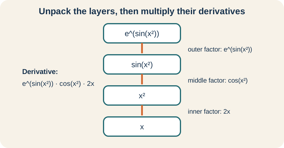
Some expressions contain several nested layers. For $e^{\sin(x^2)}$, the input is squared, sine acts on that result, and the exponential acts last. A dependency list is $x\to x^2\to\sin(x^2)\to e^{\sin(x^2)}$. Every arrow whose operation changes with its input contributes a derivative factor. Writing this list before calculating is often faster than repairing a missing factor afterward.

State the chain rule precisely

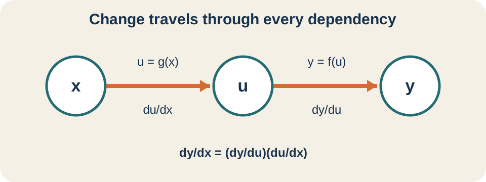
Suppose $u=g(x)$ and $y=f(u)$. If $g$ is differentiable at $x$ and $f$ is differentiable at $u=g(x)$, then $\frac{dy}{dx}=\frac{dy}{du}\frac{du}{dx}$. In function notation, the same statement is $(f\circ g)'(x)=f'(g(x))g'(x)$. The factor $f'(g(x))$ is the derivative of the outer function evaluated at the unchanged inner output. The factor $g'(x)$ is the derivative of the inner function.

The hypotheses matter because a composition can fail to be differentiable at either layer. The inner function must have a well-defined local linear approximation at the chosen input. The outer function must have one at the inner output, not merely somewhere else in its domain. These conditions explain why checking domains before and after differentiation is necessary. A symbolic rule cannot manufacture differentiability where the original relationship lacks it.

Leibniz notation makes the dependency structure visible, but the symbols do not literally cancel like ordinary numbers. The expression $\frac{dy}{du}\frac{du}{dx}$ is a product of two derivatives justified by a limit theorem. Its middle symbol $du$ suggests the matching intermediate variable. That suggestion is valuable for arranging factors and checking units. The proof, however, depends on differentiability rather than algebraic cancellation of infinitesimals.

Understand why the factors multiply

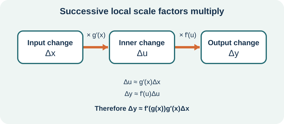
Near an input $x$, differentiability lets us approximate the inner change by $\Delta u\approx g'(x)\Delta x$. The symbol $\Delta$ means a finite change, so $\Delta x$ is the input increment and $\Delta u$ is the resulting inner increment. Near $u=g(x)$, the outer change is $\Delta y\approx f'(u)\Delta u$. Substituting the first approximation into the second gives $\Delta y\approx f'(g(x))g'(x)\Delta x$. The coefficient of $\Delta x$ is therefore the overall derivative.

This argument is local linearity in action. The inner derivative converts a small change in $x$ into a small change in $u$. The outer derivative then converts that change in $u$ into a small change in $y$. Successive conversions multiply in the same way that successive scale factors multiply. The chain rule is therefore a composition rule for local linear models.

A limit derivation makes the same logic exact. Insert the factor $\frac{g(a+h)-g(a)}{g(a+h)-g(a)}$ into the composition’s difference quotient when the inner difference is nonzero. The quotient becomes an outer difference quotient multiplied by an inner difference quotient. As $h$ approaches zero, continuity from differentiability makes the intermediate input approach $g(a)$. The two limits become $f'(g(a))$ and $g'(a)$, producing their product, with the zero-inner-change cases handled by the differentiability remainder form.

Apply the outer-then-inner procedure

Differentiate $y=(3x^2-1)^5$ by preserving the inner expression. Let $u=3x^2-1$, so $y=u^5$. The outer derivative is $\frac{dy}{du}=5u^4$, while the inner derivative is $\frac{du}{dx}=6x$. Multiplication gives $\frac{dy}{dx}=5(3x^2-1)^4(6x)$. Simplifying constants yields $y'=30x(3x^2-1)^4$.

Notice what remains unchanged during the outer step. Differentiating the fifth power lowers its exponent to four, but the complete inner expression stays inside the fourth power. Only after that step do we multiply by the derivative of the inside. Replacing the inside prematurely often destroys the composition’s structure. The verbal pattern is “derivative of the outside, evaluated at the inside, times derivative of the inside.” Say that pattern aloud while pointing to the matching factors until the structure becomes automatic.

Now differentiate $F(x)=\sqrt{1+4x^3}=(1+4x^3)^{\frac{1}{2}}$. The fractional exponent is the outer operation, and $1+4x^3$ is inner. The power rule gives $\frac{1}{2}(1+4x^3)^{-\frac{1}{2}}$, and the inner derivative is $12x^2$. Thus $F'(x)=\frac{6x^2}{\sqrt{1+4x^3}}$. This derivative is finite only where the radicand is positive, even though the original square root also exists at a zero radicand.

Differentiate exponential and logarithmic compositions

For $y=e^{x^2}$, the exponential function is outer and $x^2$ is inner. Because the derivative of $e^u$ with respect to $u$ is $e^u$, the outer factor is $e^{x^2}$. The inner derivative is $2x$. Therefore $y'=2xe^{x^2}$. The original exponential factor remains because its rate of change equals its value with respect to its own input.

For a general positive base $b$, $\frac{d}{dx}b^{g(x)}=b^{g(x)}\ln(b)g'(x)$. The symbol $\ln(b)$ is the natural logarithm of the constant base and belongs to the outer derivative. For example, $\frac{d}{dx}2^{3x}=2^{3x}\ln(2)(3)$. The factor three comes from the inner function $3x$. Omitting either constant changes the local rate.

For $y=\ln(5-x^2)$, the logarithm rule gives the reciprocal of its input times the input’s derivative. Thus $y'=\frac{1}{5-x^2}(-2x)=\frac{-2x}{5-x^2}$. The original real-valued logarithm requires $5-x^2>0$. That inequality means $-\sqrt{5}<x<\sqrt{5}$. A correct derivative statement preserves this domain rather than reporting only a formula.

Differentiate trigonometric compositions

For $y=\sin(x^2)$, sine is outer and the square is inner. The outer derivative is cosine evaluated at the same inner expression, giving $\cos(x^2)$. The inner derivative is $2x$. Therefore $y'=2x\cos(x^2)$. This standard formula assumes angles are measured in radians, because the familiar sine derivative is a radian-based limit result.

For $y=\cos(4x-1)$, the outer derivative contributes a negative sine. Keeping the inside unchanged gives $-\sin(4x-1)$. The inner derivative contributes the factor four. Hence $y'=-4\sin(4x-1)$. The negative sign and the inner factor arise from different layers and should be checked separately.

For $y=\tan^3x$, conventional notation means $[\tan(x)]^3$, not $\tan(x^3)$. The cube is outer, tangent is the next layer, and $x$ is the innermost input. Differentiation gives $3\tan^2x\sec^2x$. The expression is defined only where $\cos x\ne0$. Parsing notation correctly is part of recognizing the composition.

Manage multiple layers systematically

Consider $y=e^{\sin(x^2)}$. Begin with the outer exponential, whose derivative reproduces $e^{\sin(x^2)}$. Next differentiate the sine layer to obtain $\cos(x^2)$. Finally differentiate the square layer to obtain $2x$. Multiplying gives $y'=2xe^{\sin(x^2)}\cos(x^2)$. Each factor corresponds to one arrow in the dependency chain.

Intermediate variables make a long chain easier to audit. Set $u=x^2$, $v=\sin u$, and $y=e^v$. Then $\frac{dy}{dx}=\frac{dy}{dv}\frac{dv}{du}\frac{du}{dx}$. Substitution produces $e^v\cos u(2x)$ and then restores $u$ and $v$. This notation helps ensure that no variable is skipped or differentiated with respect to the wrong input.

The same method works for $F(x)=\sqrt{1+[\ln(x)]^2}$. The layers are square root, addition of one, squaring, logarithm, and the original input. Constant addition contributes a derivative of one and does not create a visible factor. The result is $F'(x)=\frac{\ln x}{x\sqrt{1+[\ln(x)]^2}}$. Its real domain requires $x>0$, and the denominator remains nonzero throughout that domain, including at $x=1$ where $\ln(1)=0$.

Track units through composed rates

Suppose position $s$ is measured in meters, time $t$ in seconds, and energy $E$ in joules. The sensitivity $\frac{dE}{ds}$ has units of joules per meter. The velocity $\frac{ds}{dt}$ has units of meters per second. Their product has units $\frac{\mathrm{J}}{\mathrm{m}}\frac{\mathrm{m}}{\mathrm{s}}=\frac{\mathrm{J}}{\mathrm{s}}$. These are the required units for the energy rate $\frac{dE}{dt}$.

Consider a spherical balloon with $V(r)=\frac{4}{3}\pi r^3$. If radius depends on time, the chain rule gives $\frac{dV}{dt}=\frac{dV}{dr}\frac{dr}{dt}=4\pi r^2\frac{dr}{dt}$. At $r=0.20\,\mathrm{m}$ and $\frac{dr}{dt}=0.010\,\frac{\mathrm{m}}{\mathrm{s}}$, the rate is $4\pi(0.20\,\mathrm{m})^2(0.010\,\frac{\mathrm{m}}{\mathrm{s}})$. This equals $1.6\pi\times10^{-3}\,\frac{\mathrm{m^3}}{\mathrm{s}}$. Cubic meters per second confirm that the result is a volume rate.

Units can expose a missing chain factor. The geometric derivative $4\pi r^2$ alone has square-meter units, not cubic meters per second. Multiplication by $\frac{dr}{dt}$ supplies meters per second and completes the dimensions. A numerically plausible answer with wrong dimensions is still structurally wrong. Treat dimensional analysis as an independent verification step.

Use the chain rule in implicit differentiation

An implicit equation relates variables without isolating one of them. For $x^2+y^2=25$, regard $y$ as an unknown function of $x$. Differentiating with respect to $x$ gives $2x+2y\frac{dy}{dx}=0$. The factor $\frac{dy}{dx}$ appears because differentiating $y^2$ requires the chain rule. Solving yields $\frac{dy}{dx}=-\frac{x}{y}$ where $y\ne0$.

The restriction $y\ne0$ belongs to the solved slope formula. At points $(5,0)$ and $(-5,0)$, the circle has vertical tangents, so a finite derivative with respect to $x$ does not exist. Differentiating with respect to $y$ instead gives information about $\frac{dx}{dy}$. This behavior is geometric rather than an algebraic defect. Domain and tangent orientation must accompany the formula.

For $xy+y^2=6$, use both the product rule and chain rule. Differentiation gives $y+x\frac{dy}{dx}+2y\frac{dy}{dx}=0$. Collecting derivative terms produces $(x+2y)\frac{dy}{dx}=-y$. Therefore $\frac{dy}{dx}=\frac{-y}{x+2y}$ when $x+2y\ne0$. Naming which rule creates each term prevents the common omission of $y$ from the derivative of $xy$.

Derive derivatives of inverse functions

If $f$ has a differentiable local inverse, then $f(f^{-1}(x))=x$. Differentiate both sides with respect to $x$. The chain rule gives $f'(f^{-1}(x))(f^{-1})'(x)=1$. Solving produces $(f^{-1})'(x)=\frac{1}{f'(f^{-1}(x))}$. The denominator must be nonzero at the corresponding original input.

Suppose $f(2)=5$ and $f'(2)=3$. Because $f^{-1}(5)=2$, the inverse derivative at five is $(f^{-1})'(5)=\frac{1}{f'(2)}=\frac{1}{3}$. The input five belongs to the inverse function, while two is the matching input of the original function. Confusing those coordinates is a frequent error. Thinking of inverse graphs as reflections across $y=x$ helps swap their roles correctly.

Local invertibility also matters. The function $f(x)=x^2$ has no single inverse on all real numbers because two inputs can share one output. Restricting it to $x\ge0$ produces the inverse $f^{-1}(x)=\sqrt{x}$. At the original input zero, $f'(0)=0$, so the reciprocal formula predicts no finite inverse derivative. Correspondingly, the square-root graph has a vertical tangent at zero.

Diagnose errors and verify results

The most common error is differentiating the outer function but forgetting the inner derivative. Writing $\frac{d}{dx}(x^2+1)^5=5(x^2+1)^4$ misses the factor $2x$. Another error is replacing the inside with its derivative, producing $5(2x)^4$. The correct outer step keeps the original inside intact. Only multiplication by its derivative follows afterward.

A second class of errors comes from misidentifying structure. A product such as $x^2\sin x$ needs the product rule, while $\sin(x^2)$ needs the chain rule. A quotient can contain compositions and therefore require both quotient and chain rules. Parentheses and a dependency tree reveal which rule governs each layer. Name the outermost operation before performing any algebra.

Verify a result in three ways. First, compare units whenever variables represent measured quantities. Second, check a numerical difference quotient $\frac{F(a+h)-F(a)}{h}$ for a small safe value of $h$. Third, inspect signs and rough magnitudes from the graph near $a$. Agreement among symbolic, numerical, and graphical evidence is stronger than repeated symbolic manipulation alone.

Guided synthesis and connection forward

Differentiate $G(x)=\ln(1+x^4)$. The logarithm is outer, so its derivative contributes the reciprocal $\frac{1}{1+x^4}$. The inner derivative is $4x^3$. Thus $G'(x)=\frac{4x^3}{1+x^4}$. Because $1+x^4$ is always positive for real $x$, both the original function and derivative are defined everywhere.

Now differentiate $H(x)=\cos^2(3x)$. The square is outer, cosine is the middle layer, and $3x$ is inner. The factors are $2\cos(3x)$, $-\sin(3x)$, and $3$. Their product is $H'(x)=-6\cos(3x)\sin(3x)$. The equivalent form $-3\sin(6x)$ follows from a double-angle identity, but the unsimplified form displays the chain more clearly.

For independent practice, differentiate $e^{\sqrt{1+x^2}}$, $\ln(\cos x)$ where defined, and $(2+ an x)^{-3}$. For each expression, draw or write the dependency chain before calculating. Label every derivative factor with the layer that created it. State the real domain and check one value numerically. The next applications lessons will use this same sensitivity logic in related rates, optimization models, and motion.

Sources and further study

The principal mathematical reference for this lesson is OpenStax Calculus, Volume 1. Its differentiation chapters develop the chain rule from composite functions. They also connect the rule to implicit differentiation and inverse functions. Compare its notation with the dependency notation used here. Translating between equivalent notations is a useful form of retrieval practice.

The AP Calculus AB course overview provides the curriculum alignment for these skills. It places composition analysis and the chain rule within the broader study of differentiation. Its framework also emphasizes interpreting derivatives in context. Use its topic sequence to identify which prerequisite rules need further review. Curriculum placement does not replace the mathematical hypotheses stated in this lesson.

When consulting another source, test each example by naming its layers before reading the solution. Then predict the number and kind of derivative factors that should appear. Check whether the source states relevant domain restrictions. Verify one worked result with a numerical difference quotient. Active comparison turns a reference into practice rather than passive rereading.