Partial Derivatives

A function of several variables can change at different rates in different directions. Partial derivatives isolate coordinate directions, while the gradient assembles those coordinate rates into a geometric object. Linearization then predicts small changes without pretending that a curved surface is globally flat. Units and held-fixed conditions are essential parts of every interpretation. This lesson develops computation, meaning, geometry, approximation, and error diagnosis together.

Move from a curve to a surface

A single-variable function $y=f(x)$ assigns one output to each allowed input $x$. Its graph is a curve, and its derivative measures change along the only available input direction. A two-variable function $z=f(x,y)$ assigns one output to each ordered pair $(x,y)$. Its graph is generally a surface in three-dimensional space. The extra input direction makes the phrase “the slope” incomplete until a direction is specified.

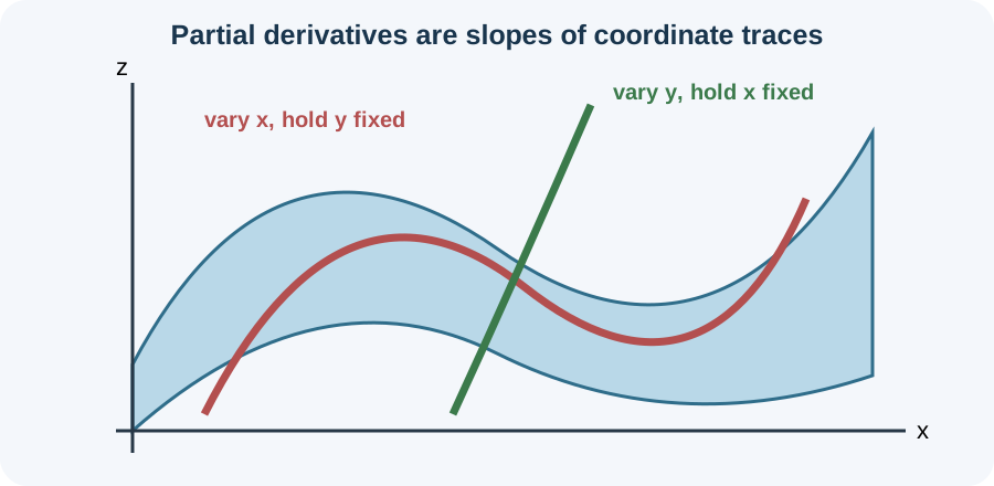
One way to study the surface is to hold $y=b$ fixed. The resulting trace $z=f(x,b)$ is an ordinary curve whose variable is $x$. Holding $x=a$ instead produces the trace $z=f(a,y)$. The slopes of these coordinate traces are partial derivatives. They answer different questions because each allows a different input to vary.

For $f(x,y)=x^2+3y^2$, movement parallel to the $x$-axis changes only the $x^2$ term. Movement parallel to the $y$-axis changes only the $3y^2$ term. Movement along a diagonal changes both terms at once. A partial derivative is therefore not a reduced version of the full change. It is one directional measurement from which broader local behavior can be assembled.

Define a partial derivative with a limit

The partial derivative of $f$ with respect to $x$ at $(a,b)$ is $f_x(a,b)=\lim_{h\to0}\dfrac{f(a+h,b)-f(a,b)}{h}$. The subscript $x$ identifies the changing coordinate. The value $b$ remains fixed in both function evaluations. The increment $h$ changes only the first coordinate, and the denominator records that input change. The quotient becomes an instantaneous coordinate rate when the limit exists.

Similarly, the partial derivative with respect to $y$ is $f_y(a,b)=\lim_{h\to0}\dfrac{f(a,b+h)-f(a,b)}{h}$. Now $a$ remains fixed and only the second coordinate changes. The same letter $h$ can be used because the two limits are separate definitions. The curved symbol $\partial$ in $\dfrac{\partial f}{\partial y}$ distinguishes partial differentiation from the ordinary derivative symbol $d$. Every notation should remind the reader which input is allowed to move.

The limit notation expresses a process rather than substitution of $h=0$. Direct substitution would create a zero denominator. Instead, nonzero increments approach zero while the quotient records average coordinate rates. If those rates approach one finite value, the partial derivative exists. This interpretation matches the ordinary derivative while imposing a held-coordinate condition. It also explains why a graph’s local coordinate trace determines the value.

Compute by treating other variables as constants

To calculate $f_x$, apply ordinary differentiation rules to $x$ while treating $y$ as a constant. For $f(x,y)=x^2y+e^{xy}$, the derivative of $x^2y$ with respect to $x$ is $2xy$. The chain rule gives the derivative of $e^{xy}$ as $ye^{xy}$. Therefore $f_x(x,y)=2xy+ye^{xy}$. The symbol $y$ remains in the answer because its fixed value selects which coordinate trace is being measured.

To calculate $f_y$, treat $x$ as a constant instead. The derivative of $x^2y$ with respect to $y$ is $x^2$. The chain rule gives the derivative of $e^{xy}$ as $xe^{xy}$. Thus $f_y(x,y)=x^2+xe^{xy}$. Comparing the two results exposes which factors arise from differentiating the inner product $xy$.

A useful verbal check accompanies each line. For $f_x$, say that $y$ is temporarily a constant coefficient. For $f_y$, say that $x$ is temporarily a constant coefficient. This language prevents the common error of differentiating every visible variable at once. Substituting the point after differentiating usually preserves structure and reduces arithmetic clutter.

Interpret signs, magnitudes, and units

Suppose temperature is $T(x,y)$, where $T$ is measured in degrees Celsius and both coordinates are measured in metres. Then $T_x$ has units of degrees Celsius per metre. A positive value means temperature increases locally when moving in the positive $x$ direction with $y$ fixed. A negative value means it decreases in that coordinate direction. A magnitude of $3\,\mathrm{^{\circ}C\,m^{-1}}$ represents about three degrees Celsius of change per metre for sufficiently small movement.

If the inputs have different units, the partial derivatives also have different units. For a cost $C(q,t)$ measured in dollars, with quantity $q$ in units and time $t$ in hours, $C_q$ has units of dollars per unit. The derivative $C_t$ has units of dollars per hour. Their numerical values should not be compared as though they measured the same kind of sensitivity. Units reveal both meaning and invalid arithmetic.

The phrase “holding other variables fixed” is a modeling condition. In thermodynamics, changing volume while holding temperature fixed describes a different process from changing volume while holding pressure fixed. The notation must make the held variables unambiguous when several state quantities are related. A derivative can be computed correctly yet interpreted for the wrong experiment. Always attach the coordinate condition and units to the reported rate.

Build the tangent plane through linearization

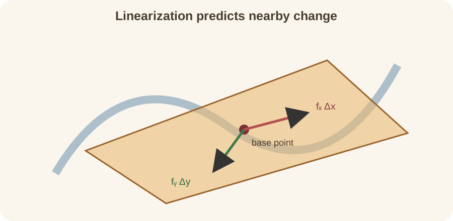
Near $(a,b)$, a differentiable function behaves approximately like a plane. Its linearization is $L(x,y)=f(a,b)+f_x(a,b)(x-a)+f_y(a,b)(y-b)$. The first term anchors the approximation at the known surface value. Each partial derivative converts its corresponding input displacement into predicted output change. Adding the two contributions produces the local planar model.

For $f(x,y)=x^2+y^2$ at $(1,2)$, the function value is $5$. The partial derivatives are $f_x=2x$ and $f_y=2y$, so their values are $2$ and $4$. The linearization is $L(x,y)=5+2(x-1)+4(y-2)$. At $(1.02,1.99)$, this predicts $5+2(0.02)+4(-0.01)=5$. The exact value is $1.02^2+1.99^2=5.0005$, illustrating small local error.

The same expression describes the tangent plane when written $z=L(x,y)$. Linearization is more than a drawing because it gives numerical estimates. It also predicts the total differential $df=f_x\,dx+f_y\,dy$. The approximation improves as the input change approaches zero when the function is differentiable. Large displacements may reveal curvature that the tangent plane cannot represent.

Separate partial existence from differentiability

The existence of $f_x(a,b)$ and $f_y(a,b)$ does not alone prove differentiability. Each partial derivative examines only one coordinate line through the point. A function can behave gently along those two lines yet change irregularly along another path. Differentiability requires one linear model to approximate changes from all nearby directions. This is a stronger demand than two isolated one-dimensional limits.

A common sufficient condition is continuity of the first partial derivatives in a neighborhood of the point. If $f_x$ and $f_y$ exist nearby and are continuous at $(a,b)$, then $f$ is differentiable there. This theorem is sufficient rather than necessary. Some differentiable functions have partial derivatives that fail to be continuous. The theorem is valuable because continuity is often easier to verify than the full definition.

When a formula changes by cases, test more than coordinate axes. Approach the point along lines such as $y=mx$, along curves, or through polar coordinates when appropriate. Different limiting behavior along two paths disproves continuity and therefore disproves differentiability. Matching a few paths cannot by itself prove a multivariable limit. The logical asymmetry is important: disagreement disproves, while agreement merely supplies evidence.

Assemble coordinate rates into the gradient

For a scalar function $f(x,y)$, the gradient is $\nabla f=\langle f_x,f_y\rangle$. The symbol $\nabla$ is read “del” or “nabla.” Angle brackets indicate a vector whose components are the coordinate partial derivatives. In three variables, $\nabla f=\langle f_x,f_y,f_z\rangle$. The gradient depends on position because its components usually depend on the inputs. Evaluating the gradient at a point produces a numerical vector anchored at that point.

The gradient packages local sensitivity into one vector. Its first component predicts change per unit movement in the $x$ direction. Its second component does the same for $y$, and a third component does so for $z$ when present. This packaging allows vector algebra to describe arbitrary directions. The gradient is not the graph of the function and should not be confused with a point on its surface.

For $f(x,y)=x^2+3y^2$, the gradient is $\nabla f=\langle2x,6y\rangle$. At $(1,2)$, it becomes $\langle2,12\rangle$. The vector has a much larger positive $y$ component, indicating greater local sensitivity to positive $y$ motion. Its magnitude is $\sqrt{2^2+12^2}=\sqrt{148}$. Magnitude and direction together summarize the strongest first-order change.

Measure change in an arbitrary direction

Let $\mathbf u$ be a unit vector specifying a direction. The directional derivative is $D_{\mathbf u}f(a,b)=\nabla f(a,b)\cdot\mathbf u$. The dot denotes the vector dot product. Each component weights a coordinate rate by how much the direction points along that coordinate. Requiring unit length makes the result a rate per unit distance.

For $f(x,y)=x^2+3y^2$ at $(1,2)$, use direction $\mathbf u=\left\langle\dfrac{3}{5},\dfrac{4}{5}\right\rangle$. Its length is one because $\sqrt{(3/5)^2+(4/5)^2}=1$. The directional derivative is $\langle2,12\rangle\cdot\left\langle\dfrac{3}{5},\dfrac{4}{5}\right\rangle=\dfrac{54}{5}$. This value measures the predicted increase in $f$ per unit distance along that direction. Reversing the direction changes the sign but not the magnitude.

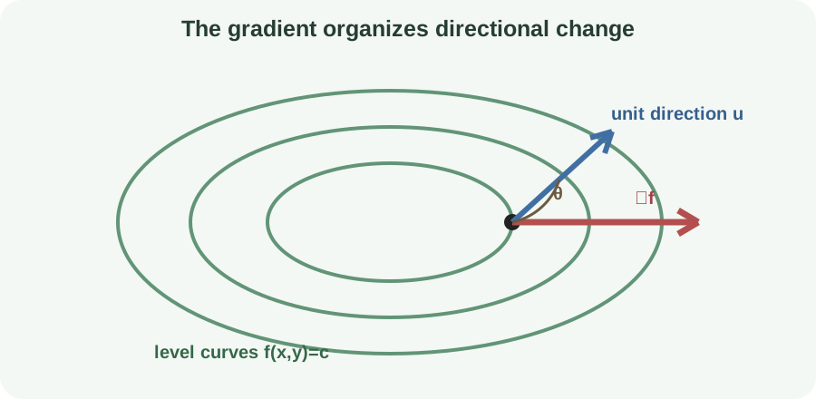
The dot-product formula gives $D_{\mathbf u}f=\|\nabla f\|\cos\theta$, where $\theta$ is the angle between the two vectors. The maximum occurs when $\cos\theta=1$, so the gradient points toward steepest increase. The minimum occurs in the opposite direction. A perpendicular direction has zero first-order change and is tangent to a level curve. This geometric result follows directly from the dot product rather than from a separate rule.

Connect gradients with level curves and surfaces

A level curve of $f(x,y)$ is a set satisfying $f(x,y)=c$ for a constant $c$. Every point on that curve has the same function value. Motion tangent to the curve therefore produces zero instantaneous change in $f$. The directional derivative along a tangent vector is zero. Consequently, a nonzero gradient is perpendicular to the level curve.

For $f(x,y)=x^2+3y^2$, level curves satisfy $x^2+3y^2=c$. These curves are ellipses when $c>0$. At $(1,2)$, the gradient $\langle2,12\rangle$ points normal to the ellipse passing through that point. A tangent vector has dot product zero with this gradient. The orthogonality links algebraic derivatives to visible contour geometry.

In three variables, a level surface satisfies $F(x,y,z)=c$. The gradient $\nabla F$ is normal to the surface when it is nonzero. This fact helps construct tangent planes to implicitly defined surfaces. It also underlies normal vectors in flux integrals and constrained optimization. Level-set geometry is one of the most reusable interpretations of partial derivatives.

Apply the multivariable chain rule

Suppose $z=f(x,y)$ while $x=x(t)$ and $y=y(t)$ depend on time. The chain rule is $\dfrac{dz}{dt}=f_x\dfrac{dx}{dt}+f_y\dfrac{dy}{dt}$. Every partial derivative is evaluated at the current point $(x(t),y(t))$. Each coordinate contribution is converted into output change and then added. The formula matches $\nabla f\cdot\mathbf r'(t)$ and does not require unit speed.

Let $f(x,y)=x^2y$, with $x=t^2$ and $y=3t+1$. The partial derivatives are $f_x=2xy$ and $f_y=x^2$. The input rates are $dx/dt=2t$ and $dy/dt=3$. Hence $dz/dt=(2xy)(2t)+(x^2)(3)$. Substituting $x=t^2$ and $y=3t+1$ yields a result entirely in terms of time.

A dependency diagram can prevent omitted terms. Draw arrows from $t$ to both $x$ and $y$, then arrows from those variables to $z$. Every path from $t$ to $z$ contributes a product of derivatives along that path. When intermediate variables share dependencies, the sum contains all routes of influence. This viewpoint scales to models with many inputs and parameters.

Compute second partial derivatives and the Hessian

Differentiating a first partial again produces a second partial. The notation $f_{xx}$ means differentiate twice with respect to $x$. The mixed partial $f_{xy}$ means first differentiate with respect to $x$ and then the resulting expression with respect to $y$. Some textbooks reverse the verbal convention, so the displayed operations should control interpretation. Writing $\partial^2f/(\partial y\,\partial x)$ makes the order explicit.

For $f(x,y)=x^2y+e^{xy}$, one can compute $f_{xx}$, $f_{xy}$, $f_{yx}$, and $f_{yy}$. Under suitable continuity assumptions, the mixed partials satisfy $f_{xy}=f_{yx}$. This equality is a theorem, not a typographical rule. Functions with insufficient smoothness can violate it at special points. Checking assumptions prevents an unwarranted interchange of differentiation order.

The Hessian matrix collects second partial derivatives. In two variables it is $H_f=\begin{pmatrix}f_{xx}&f_{xy}\\f_{yx}&f_{yy}\end{pmatrix}$. Diagonal entries measure curvature along coordinate directions. Off-diagonal entries describe how one coordinate rate changes as another coordinate changes. The Hessian refines the first-order information supplied by the gradient.

Locate and interpret critical points

At an interior differentiable local maximum or minimum, the gradient must be zero. Such a point satisfies $\nabla f=\mathbf0$, where the bold zero is the zero vector. Points where derivatives fail to exist can also be critical candidates. Solving the gradient equations generates candidates rather than proving extrema. Boundary points require separate analysis because movement in every direction may not be allowed.

For $f(x,y)=x^2+3y^2$, the gradient vanishes only at $(0,0)$. The function is nonnegative and equals zero there, so the point is a global minimum. That conclusion follows directly from the formula, not merely from the zero gradient. For a saddle such as $f(x,y)=x^2-y^2$, the gradient also vanishes at the origin. Opposite curvature directions prevent an extremum.

The Hessian can classify an isolated critical point when its second-derivative test is conclusive. Positive curvature in every direction indicates a local minimum, while negative curvature in every direction indicates a local maximum. Mixed signs indicate a saddle. An inconclusive Hessian does not imply that no classification exists. It means higher-order reasoning or direct inequalities are needed.

Estimate uncertainty with differentials

Linearization estimates how input uncertainty propagates into output uncertainty. For small changes, $\Delta f\approx f_x\Delta x+f_y\Delta y$. The delta symbol $\Delta$ denotes a finite change, while the differential expression represents its first-order approximation. Signs matter when changes are known and coordinated. For worst-case bounds, magnitudes are often added instead.

Suppose a rectangular area is $A=LW$, with measured length and width in metres. The partial derivatives are $A_L=W$ and $A_W=L$. Small measurement changes give $\Delta A\approx W\Delta L+L\Delta W$. Each term has units of square metres because metres multiply metres. Unit consistency confirms that the approximation can be added to an area.

If only uncertainty bounds are known, then $|\Delta A|\lesssim |W|,|\Delta L|+|L|,|\Delta W|$. The symbol $\lesssim$ communicates an approximate upper bound rather than exact equality. Statistical uncertainty propagation may combine independent contributions differently, often through squared terms. The choice depends on what the uncertainty statements mean. Partial derivatives supply sensitivities, while the uncertainty model determines how they are combined.

Diagnose mistakes and practice deliberately

One common mistake is differentiating a variable that should be held fixed. Another is substituting a point before the symbolic structure is clear. A third is using a direction vector without normalizing it. A fourth is assuming that existing partials prove differentiability. State the changing variable and held-fixed variables before each computation to prevent these errors.

Practice first with $f(x,y)=x^3y+\sin y$. Compute $f_x=3x^2y$ and $f_y=x^3+\cos y$, explaining why the sine term disappears only from $f_x$. Then evaluate both at a chosen point and attach units from an invented physical context. Construct the tangent plane at that point. Compare its prediction with the exact function at one nearby input.

Next use $g(x,y)=xe^y$ at $(2,0)$. Its gradient is $\langle e^y,xe^y\rangle$, which becomes $\langle1,2\rangle$. The unit direction of steepest increase is $\left\langle\dfrac{1}{\sqrt5},\dfrac{2}{\sqrt5}\right\rangle$. Verify that this vector has length one. Finally, choose a perpendicular direction and confirm that its directional derivative is zero.

Connect forward to multivariable accumulation

Partial derivatives describe local change, while multiple integrals accumulate quantities over regions. The two ideas interact through the multivariable fundamental theorems. Coordinate changes introduce Jacobian derivatives that measure local stretching. Optimization uses gradients to identify candidates and constraints to restrict directions. Differential equations use partial derivatives when unknown quantities depend on space and time.

In data fitting, a model may depend on many adjustable parameters. Partial derivatives measure how each predicted value changes when one parameter varies. Collecting those derivatives produces a Jacobian matrix. Gauss–Newton and Levenberg–Marquardt methods use that matrix to choose parameter updates. The coordinate-rate idea from this lesson therefore supports practical nonlinear optimization.

You are ready to proceed when you can compute a partial derivative and narrate what remains fixed. You should interpret units, construct a linearization, normalize directions, and connect gradients with level curves. You should distinguish partial existence from differentiability and a critical candidate from a proven extremum. These distinctions make the notation carry meaning rather than merely instructions. Multiple integrals can then add accumulation to this local-change foundation.