Multiple Integrals

A multiple integral accumulates a quantity distributed across a two-dimensional or three-dimensional region. The integrand describes density per unit area or volume, while the differential element describes a small geometric piece. Riemann sums explain why those factors multiply and then add. Iterated integrals convert multidimensional accumulation into a sequence of one-variable integrations. Coordinate changes reshape difficult regions, but their Jacobian factors must preserve local area or volume.

Extend one-dimensional accumulation to a region

A single integral accumulates values across small intervals of width $\Delta x$. A double integral accumulates across small pieces of area $\Delta A$. A triple integral accumulates across small pieces of volume $\Delta V$. The dimensionality of the domain changes, but the pattern remains density times small measure followed by summation. Understanding that pattern is more durable than memorizing several integral symbols.

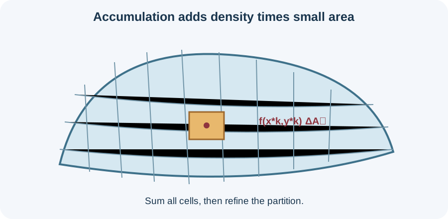
Let $R$ be a bounded region in the $xy$-plane. Partition it into small subregions $R_k$ with areas $\Delta A_k$. Choose a sample point $(x_k^*,y_k^*)$ inside each piece. The sum $\sum_k f(x_k^*,y_k^*)\Delta A_k$ approximates the total accumulation. The subscript $k$ indexes pieces rather than representing a coordinate.

As the largest subregion diameter approaches zero, the Riemann sums may approach a unique limit. That limit is written $\iint_R f(x,y)\,dA$. The double integral symbol signals accumulation over a planar region. The differential $dA$ represents an infinitesimal area element. Existence requires appropriate behavior from both the function and the region.

Interpret what a double integral measures

If $f(x,y)\geq0$ represents height above the $xy$-plane, then $\iint_R f\,dA$ represents volume under the surface. Each product $f\Delta A$ approximates a thin column. Adding the columns approximates total volume. The limiting process removes dependence on the particular partition. This geometric interpretation is useful but not universal.

If $f$ can be negative, the integral is signed accumulation. Contributions below zero subtract from contributions above zero. The result need not equal geometric volume because geometric volume is nonnegative. If $f$ is surface mass density, the integral gives mass rather than volume. Interpretation comes from the integrand and its units.

Suppose surface density $\sigma$ has units $\mathrm{kg\,m^{-2}}$. The area element has units $\mathrm{m^2}$. Their product has units $\mathrm{kg}$, so $\iint_R\sigma\,dA$ is mass. Unit multiplication explains the physical meaning before evaluation. A correct antiderivative with incorrect units signals a flawed setup or model.

Convert a rectangular region into an iterated integral

For rectangle $R=[a,b]\times[c,d]$, a double integral can be evaluated as $\int_a^b\int_c^d f(x,y)\,dy\,dx$. The inner integral treats $x$ as fixed and accumulates in the $y$ direction. Its result is then a function of $x$. The outer integral accumulates those strip totals from $a$ to $b$. Read the differentials from inside outward to identify the order.

Under conditions supplied by Fubini’s theorem, the order can be reversed: $\int_a^b\int_c^d f\,dy\,dx=\int_c^d\int_a^b f\,dx\,dy$. Continuity on a closed rectangle is a familiar sufficient condition. More general integrability conditions also exist. Order exchange is a theorem-supported operation rather than a typographical rearrangement. The bounds must move with their corresponding variables.

For $f(x,y)=x+2y$ on $0\leq x\leq1$ and $0\leq y\leq2$, integrate in $y$ first. The inner result is $\int_0^2(x+2y)\,dy=2x+4$. Integrating from $x=0$ to $x=1$ gives $\int_0^1(2x+4)\,dx=5$. Reversing order gives the same value and supplies an independent check. The agreement also confirms that both descriptions cover the identical rectangle.

Describe variable-bound regions with slices

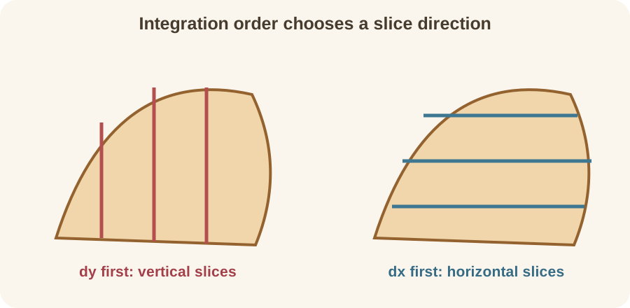
A Type I region uses vertical slices: $R=\{(x,y):a\leq x\leq b,\ g_1(x)\leq y\leq g_2(x)\}$. For each fixed $x$, the variable $y$ runs from a lower boundary to an upper boundary. The corresponding integral is $\int_a^b\int_{g_1(x)}^{g_2(x)}f(x,y)\,dy\,dx$. The outer bounds cover the horizontal shadow of the region. Every vertical slice should enter and leave the region exactly once.

A Type II region uses horizontal slices: $R=\{(x,y):c\leq y\leq d,\ h_1(y)\leq x\leq h_2(y)\}$. Its integral is $\int_c^d\int_{h_1(y)}^{h_2(y)}f(x,y)\,dx\,dy$. Now the outer bounds cover the vertical shadow. The inner limits describe left and right boundaries. A region may be simple in one orientation and require splitting in the other.

Always sketch the region before writing bounds. Mark intersection points and decide which variable is swept inside. Trace several representative slices across the drawing. The inner lower and upper limits must match the slice endpoints. This geometric procedure prevents bounds that describe a different region while looking algebraically plausible.

Reverse integration order carefully

Changing order means redescribing the same set of points. It does not merely mean swapping $dx$ and $dy$. Begin from the original inequalities and draw their region. Determine the new outer interval from the region’s projection. Then solve boundaries for the new inner variable.

Consider $0\leq x\leq1$ and $x^2\leq y\leq x$. This region lies between $y=x^2$ and $y=x$. Its vertical-slice integral is $\int_0^1\int_{x^2}^{x}f(x,y)\,dy\,dx$. For horizontal slices, $0\leq y\leq1$ and $y\leq x\leq\sqrt y$. Therefore the reversed integral is $\int_0^1\int_y^{\sqrt y}f(x,y)\,dx\,dy$.

Test the new bounds with an interior point such as $(0.5,0.3)$. It satisfies $0.3\leq0.5\leq\sqrt{0.3}$. Test a point outside to ensure it is rejected. Comparing the boundary intersection values confirms the outer endpoints. These checks are faster than discovering a wrong region after lengthy integration.

Compute mass and moments from density

For a lamina occupying region $R$ with surface density $\sigma(x,y)$, mass is $M=\iint_R\sigma\,dA$. A lamina is an idealized thin plate. Density may vary with position. The mass element is $dm=\sigma\,dA$. Integration adds all infinitesimal mass contributions.

Moments about the axes are $M_x=\iint_R y\sigma\,dA$ and $M_y=\iint_R x\sigma\,dA$. The coordinate multiplying density is the perpendicular distance from the corresponding axis. These quantities have units of mass times length. The centroid is $\bar x=M_y/M$ and $\bar y=M_x/M$. Dividing by total mass produces coordinates with units of length.

Suppose $0\leq y\leq x\leq1\,\mathrm m$ and $\sigma(x,y)=(x+y)\,\mathrm{kg\,m^{-3}}$. Because $x+y$ has units of metres, the density has units $\mathrm{kg\,m^{-2}}$. The mass is $M=\int_0^{1\,\mathrm m}\int_0^x(x+y)\,\mathrm{kg\,m^{-3}}\,dy\,dx=0.500\,\mathrm{kg}$. Every bound and factor retains units. The result’s kilograms confirm density times area.

Use average value over a region

The average value of $f$ over region $R$ is $f_{\mathrm{avg}}=\dfrac{1}{\operatorname{Area}(R)}\iint_R f\,dA$. The denominator is the region’s area. The numerator is total accumulation. Their ratio has the same units as $f$. This is the multidimensional counterpart of average value on an interval.

If $f$ is temperature in degrees Celsius, integrating $f\,dA$ produces degree-Celsius square metres. Dividing by square metres returns degrees Celsius. The average is not generally the value at the geometric center. Spatial variation and region shape both affect it. Symmetry may simplify the result when the function and region have compatible patterns.

The area itself is found by integrating one: $\operatorname{Area}(R)=\iint_R1\,dA$. The integrand one is dimensionless. Multiplication by $dA$ supplies area units. This identity makes denominator construction systematic. It also provides a basic test for any proposed bounds.

Introduce polar coordinates for circular geometry

Polar coordinates describe a point by radius $r$ and angle $\theta$. The transformations are $x=r\cos\theta$ and $y=r\sin\theta$. Radius measures distance from the origin, while angle is measured from the positive $x$-axis. Also, $x^2+y^2=r^2$. Circular boundaries often become constant radial limits.

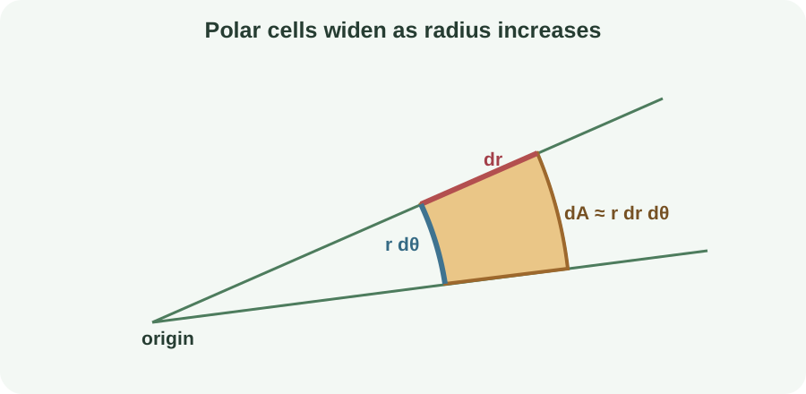
A small polar cell is approximately a thin sector. Its radial width is $dr$. Its tangential length is approximately $r\,d\theta$. Multiplying gives area element $dA=r\,dr\,d\theta$. The factor $r$ is essential because cells at larger radius span more area for the same coordinate increments.

For the disk $x^2+y^2\leq R^2$, use $0\leq r\leq R$ and $0\leq\theta\leq2\pi$. Its area is $\int_0^{2\pi}\int_0^R r\,dr\,d\theta=\pi R^2$. Omitting $r$ would produce units of length rather than area. The familiar disk formula therefore validates both the bounds and Jacobian factor. This benchmark should be checked whenever polar area notation still feels unfamiliar.

Transform integrands and bounds together

Changing to polar coordinates requires transforming every occurrence of $x$ and $y$. For example, $x^2+y^2$ becomes $r^2$. The region boundaries must also be rewritten in $r$ and $\theta$. Finally, $dA$ becomes $r\,dr\,d\theta$. Missing any one of these steps creates a mixed-coordinate expression.

Consider integrating $x^2+y^2$ over the disk of radius $R$. Polar form gives $\int_0^{2\pi}\int_0^R r^2(r\,dr\,d\theta)$. The first $r^2$ comes from the function, while the additional $r$ comes from area scaling. The radial integrand is therefore $r^3$. Keeping those origins separate prevents an unexplained exponent.

Angular bounds need not cover a complete circle. A first-quadrant disk uses $0\leq\theta\leq\dfrac{\pi}{2}$. An annulus uses inner and outer radial bounds. A sector combines angular and radial restrictions. Drawing rays and circles makes these bounds easier to verify than translating inequalities blindly.

Generalize with a Jacobian determinant

Suppose $x=x(u,v)$ and $y=y(u,v)$. The transformation maps a small rectangle in the $uv$-plane to an approximate parallelogram in the $xy$-plane. Its local area scale is the absolute Jacobian determinant. Thus $dA=\left|\dfrac{\partial(x,y)}{\partial(u,v)}\right|du\,dv$. The absolute value keeps geometric area nonnegative.

The determinant is $\dfrac{\partial x}{\partial u}\dfrac{\partial y}{\partial v}-\dfrac{\partial x}{\partial v}\dfrac{\partial y}{\partial u}$. Each partial derivative measures local stretching or shearing. The determinant combines those directional effects into oriented area scale. A negative determinant reverses orientation. Its absolute magnitude supplies the area multiplier.

For polar coordinates, the determinant equals $r$. This recovers the familiar polar area element rather than introducing an unrelated rule. A zero Jacobian signals local collapse of area and possible failure of one-to-one coordinates. Transformations should be checked for coverage and duplication. A correct determinant cannot repair bounds that traverse the region multiple times.

Extend accumulation to three dimensions

A triple integral $\iiint_E f(x,y,z)\,dV$ accumulates over a spatial region $E$. The volume element $dV$ represents a small three-dimensional piece. If $f$ is volume density in $\mathrm{kg\,m^{-3}}$, the result has units kilograms. If $f=1$, the result is the volume of $E$. Iterated integration evaluates one coordinate at a time.

Cartesian volume element is $dV=dx\,dy\,dz$ in one chosen order. Cylindrical coordinates use $x=r\cos\theta$, $y=r\sin\theta$, and $z=z$, giving $dV=r\,dr\,d\theta\,dz$ up to order. The polar area factor remains because horizontal cross-sections are circular. Bounds should describe the solid without gaps or repeated coverage. Different orders may simplify different boundary surfaces.

Standard spherical coordinates use radial distance $\rho$, polar angle $\phi$, and azimuthal angle $\theta$. Their volume element is $dV=\rho^2\sin\phi\,d\rho\,d\phi\,d\theta$. The symbol $\rho$ is a coordinate and should not be confused with a density function using the same letter. State the convention because some disciplines swap angular names. The Jacobian factor captures how spherical coordinate cells expand with radius and latitude.

Diagnose setup and evaluation errors

One common error is writing bounds without drawing the region. Another is attaching bounds to the wrong differential. A third is changing coordinates but omitting the Jacobian. A fourth is interpreting every double integral as volume. Naming the density, domain, and desired accumulated quantity prevents these category errors.

Dimensional analysis should accompany every physical integral. Density times area must produce mass for a lamina. Density times volume must produce mass for a solid. A probability density times its domain measure must produce a dimensionless probability. If units disagree, inspect the density definition, coordinate conversion, and differential element.

Numerical reasonableness also matters. Integrating a nonnegative function over a positive-area region cannot produce a negative result. An average value should lie between the minimum and maximum when those exist. Symmetric odd contributions may cancel. Estimates using minimum times area and maximum times area can bracket many answers.

Practice complete setups before calculating

For region $0\leq x\leq2\,\mathrm m$ and $x\leq y\leq2x$, sketch several vertical slices. Set up $\iint_R(x+y)\,dA$ in the stated order. Identify the units required for $x+y$ if the result is meant to be volume. Reverse the order by solving the boundary lines for $x$. Split the new description if one horizontal formula cannot cover the entire region.

For the unit disk, write $\iint_R1\,dA$ in polar coordinates. Explain why the radial bound is zero to one and the angular bound is zero to $2\pi$. Include the factor $r$. Evaluate to obtain $\pi$ square units. Then modify the bounds for the upper half-disk without changing the Jacobian.

Finally, choose a volume density of $5.00\,\mathrm{kg\,m^{-3}}$ inside a rectangular solid measuring $2.00\,\mathrm m$ by $3.00\,\mathrm m$ by $4.00\,\mathrm m$. Set up a triple integral with units. Its result is $120\,\mathrm{kg}$. Confirm the same value by density times volume. Agreement links the integral to familiar constant-density reasoning.

Connect forward to vector calculus

Multiple integrals accumulate scalar densities across regions. Vector calculus extends accumulation to circulation along curves and flux through surfaces. Orientation then affects signs as well as magnitudes. Jacobians and parameterizations describe local length, area, and volume scaling. The geometric discipline practiced here carries directly into those theorems.

Probability also uses multiple integrals for joint continuous distributions. A joint density integrates to one over its support. Integrating over a subregion gives event probability. Marginal densities arise by integrating out unwanted variables. The same bounds-and-units reasoning prevents probability errors.

You are ready to continue when you can explain a double integral as a Riemann-sum limit, build bounds from a sketch, and reverse order without changing the region. You should transform integrand, bounds, and differential element together. You should interpret Jacobians as local scale factors and attach units to physical accumulations. These habits turn multiple integration into geometry-guided accounting. Vector and probability applications can then reuse the framework with confidence.