Functions: Machines, Maps, and Relationships

A function describes dependable assignment rather than merely calculation. Once an allowed input is chosen, the function assigns exactly one output. A formula can perform that assignment, but a table, graph, algorithm, or verbal rule can do the same work. Different inputs may lead to one shared output without causing a problem. The forbidden situation is one input receiving two competing outputs from the same function.

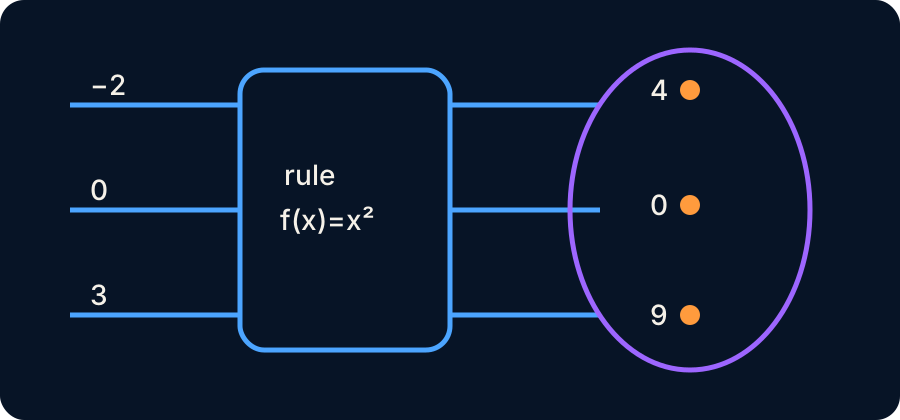
The familiar machine metaphor captures part of this idea. An input enters, a rule acts, and an output emerges. The metaphor helps learners separate the object being entered from the operation being performed. It also suggests why the same input should produce the same result whenever the rule is unchanged. However, a mathematical function need not involve time, physical machinery, or a calculable formula.

The map viewpoint is therefore more complete. It asks which inputs belong to the domain, which outputs are permitted by the codomain, and which outputs are actually reached. It also exposes composition, reversibility, and the meaning of equality between functions. These structures support limits, derivatives, integrals, scientific models, and computer programs. Learning functions well means learning to track both an assignment and the set structure surrounding it.

A function is a structured assignment

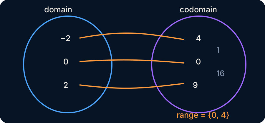
Write $f:A\to B$ to say that the function named $f$ maps from set $A$ to set $B$. The set $A$ is the domain, containing every allowed input. The set $B$ is the codomain, containing the outputs the function is declared to use. For each $x\in A$, the notation $f(x)$ names the unique element of $B$ assigned to $x$. The symbol $\in$ means “is an element of,” while the arrow records the direction of assignment.

The range is the subset of the codomain that the function actually reaches. Consider $f:\mathbb{R}\to\mathbb{R}$ defined by $f(x)=x^2$, where $\mathbb{R}$ is the set of real numbers. Its domain and codomain are both $\mathbb{R}$, but its range is $[0,\infty)$. Negative codomain values are permitted as members of $\mathbb{R}$ yet never produced by squaring a real input. Declaring $f:\mathbb{R}\to[0,\infty)$ preserves the calculation but changes the mapping claim.

A function can also be represented as a set of ordered pairs. The set $\{(1,4),(2,4),(3,9)\}$ is functional because no first coordinate receives two second coordinates. Repeated second coordinates are allowed, which is why both $1$ and $2$ may map to $4$. The set $\{(1,4),(1,7),(3,9)\}$ is not a function of the first coordinate because input $1$ has conflicting outputs. This uniqueness requirement distinguishes a function from a general relation.

Domain, codomain, and equality

A formula without a domain gives incomplete information. The expression $\frac{1}{x}$ is undefined at $x=0$, so its natural real domain excludes zero. The expression $\sqrt{x-1}$ requires $x\geq1$ when outputs are restricted to real numbers. Context can impose additional limits, such as time $t\geq0\ \mathrm{s}$ or measured temperatures between $250\ \mathrm{K}$ and $350\ \mathrm{K}$. These restrictions remain part of the function even when algebra does not display them.

Two functions are equal only when their domains agree and their outputs agree at every domain input. Define $f(x)=\frac{x^2-1}{x-1}$ on its natural domain $x\ne1$, and define $g(x)=x+1$ for every real $x$. Factoring gives $x^2-1=(x-1)(x+1)$, so $f(x)=g(x)$ wherever $x\ne1$. Nevertheless, $f$ and $g$ are not identical functions because $g(1)$ exists while $f(1)$ does not. Equality of formulas on shared inputs does not erase a difference in domains.

Preserving restrictions prevents algebraic simplification from silently changing an object. The simplified expression $x+1$ correctly describes the nearby values used to find $\lim_{x\to1}f(x)$, but it does not restore the missing input automatically. A continuous extension can be created by defining a new function with value $2$ at $x=1$. That new function agrees with $f$ on the old domain and fills the removable hole. Calculus depends on keeping nearby behavior and point membership logically separate.

Functions, equations, and graphs

An expression, an equation, and a function are related but different objects. The expression $x^2+3$ names a quantity but does not by itself declare an input set, output set, or assignment name. The equation $y=x^2+3$ describes ordered pairs satisfying a relationship. Adding a domain and codomain allows that relationship to define a function such as $f:\mathbb{R}\to\mathbb{R}$. Precise language prevents every visible formula from being called a function without qualification.

The equation $x^2+y^2=25$ describes a circle of radius $5$ in coordinate units. It does not define all of $y$ as a function of $x$ because most inputs between $-5$ and $5$ correspond to two outputs. Solving yields $y=\sqrt{25-x^2}$ and $y=-\sqrt{25-x^2}$, which are two separate functions on $[-5,5]$. Alternatively, the parameter $t$ can define the entire circle through $x(t)=5\cos t$ and $y(t)=5\sin t$. Changing the chosen input changes the functional description without changing the geometric curve.

The vertical-line test is a graphical form of output uniqueness. A plotted relation represents $y$ as a function of $x$ exactly when every vertical line intersects it at most once. Passing this test does not prove that different inputs have different outputs, because that stronger property concerns one-to-one behavior. The test also cannot infer hidden domain points beyond what the graph or problem specifies. A sideways parabola may fail as $y=f(x)$ while succeeding as $x=g(y)$.

Representations and the machine metaphor

A formula supports exact manipulation, while a table preserves selected values. A graph reveals trends, extrema, discontinuities, and asymptotic behavior. A verbal rule communicates context, assumptions, and the meaning of variables. An algorithm may define a valid assignment even when no convenient closed formula exists. Understanding improves when learners translate among these representations and ask what each one reveals or hides.

Suppose a model assigns medication amount $D$ in milligrams from body mass $m$ in kilograms by $D(m)=\min(5m,300)$. The coefficient has unit $\frac{\mathrm{mg}}{\mathrm{kg}}$, so $5m$ has unit milligrams. The minimum operation applies a maximum modeled amount of $300\ \mathrm{mg}$. A graph displays the change from proportional growth to a horizontal plateau. The verbal statement must still specify the defensible mass domain and clinical assumptions.

The machine metaphor can obscure several facts. It may suggest that every function has an executable recipe, that the codomain is irrelevant, or that output is produced after input in physical time. It can also hide functions whose elements are vectors, sets, other functions, or geometric objects. The mapping viewpoint keeps the uniqueness insight while removing those unnecessary implications. A mature understanding uses the machine as an introductory picture rather than the final definition.

Composition builds layered dependence

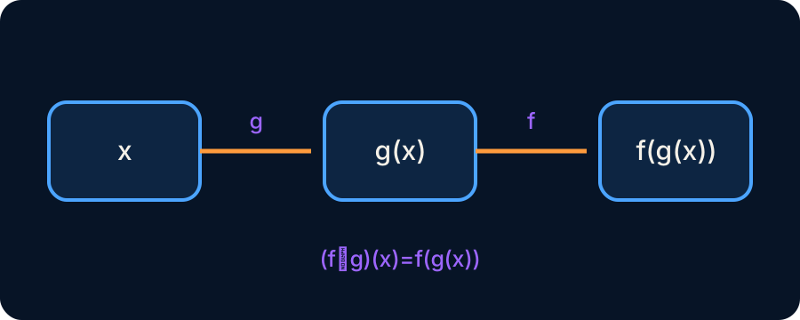
Composition connects assignments by sending the output of one function into another. If $g$ maps time $t$ in seconds to temperature $T$ in kelvins, and $f$ maps temperature to resistance $R$ in ohms, then $(f\circ g)(t)=f(g(t))$. The symbol $\circ$ denotes composition, and the inner function $g$ acts first. The composite maps time directly to resistance while retaining the intermediate physical meaning. Tracking the intermediate variable makes unit conversions and calibration assumptions visible.

Composition requires compatibility between the inner range and outer domain. If the calibration $f$ is validated only from $250\ \mathrm{K}$ through $350\ \mathrm{K}$, then every used value of $g(t)$ must remain in that interval. A symbolic formula may accept temperatures outside the calibration range without making the scientific model trustworthy there. The domains of $f\circ g$ and $g\circ f$ can therefore differ. Order records causal or logical dependence and generally cannot be reversed.

Composition is not multiplication. For $f(u)=u^2$ and $g(x)=x+1$, the composite is $(f\circ g)(x)=(x+1)^2$. The product is instead $f(x)g(x)=x^2(x+1)$. These expressions have different values, graphs, and calculus rules. Products lead to the Product Rule, whereas nontrivial compositions lead to the Chain Rule.

Inverse relationships and reversibility

An inverse function reverses an assignment. If $f:A\to B$ has inverse $f^{-1}:B\to A$, then $f^{-1}(f(x))=x$ for every $x\in A$. The superscript $-1$ indicates inverse mapping rather than reciprocal multiplication. A genuine inverse requires every relevant output to identify exactly one original input. This requirement combines one-to-one behavior with an appropriate codomain.

Squaring on all real numbers is not reversible because $2$ and $-2$ both produce $4$. Restricting the domain to $[0,\infty)$ makes $f(x)=x^2$ one-to-one and gives inverse $f^{-1}(y)=\sqrt{y}$. The inverse domain is the original range, and the inverse range is the original domain. A domain restriction is therefore not cosmetic. It records which branch of a many-to-one relationship is being reversed.

Inverse notation also clarifies scientific calibration. A sensor function may map temperature in kelvins to voltage in volts, while an inverse calibration maps voltage back to estimated temperature. Noise, rounding, or saturation can make the practical relationship only approximately invertible. The mathematical inverse describes the idealized model under stated restrictions. Measurements require an uncertainty analysis beyond symbolic reversal.

Functions prepare the language of calculus

A limit studies the outputs of a function near an input without requiring the function to be defined at that input. Continuity asks whether the limiting behavior agrees with the assigned point value. A derivative measures how output changes locally relative to input change. An integral accumulates function values over an interval. These ideas act on relationships, not merely on strings of algebraic symbols.

Units reveal the meaning of these operations. If position $s(t)$ is measured in metres and time $t$ in seconds, then a derivative $\frac{\mathrm{d}s}{\mathrm{d}t}$ has unit $\frac{\mathrm{m}}{\mathrm{s}}$. If power $P(t)$ is measured in watts, integrating over seconds produces energy in joules because $1\ \mathrm{W}=1\ \frac{\mathrm{J}}{\mathrm{s}}$. Composition propagates units through intermediate functions. A dimensionally inconsistent chain signals an invalid model or conversion.

The central lesson is that a function packages allowed inputs, permitted outputs, and a unique assignment. Formulas, graphs, tables, and machines are representations of that structure rather than substitutes for it. Domains survive simplification, codomains affect mapping claims, and composition requires compatibility. Inverses require reversible dependence on a chosen domain. With these distinctions secure, calculus can investigate how a relationship behaves, changes, and accumulates.

Piecewise rules, parameters, and modeling choices

A function may use different formulas on different parts of its domain, and such a piecewise definition is still one coherent assignment. For example, a garage might charge $C(t)=5\,\mathrm{USD}$ for $0<t\leq 1\,\mathrm{h}$ and $C(t)=5\,\mathrm{USD}+3\,\frac{\mathrm{USD}}{\mathrm{h}}(t-1\,\mathrm{h})$ for $t>1\,\mathrm{h}$. The variable $t$ denotes parking time, while $C(t)$ denotes cost, so the units clarify which quantities may sensibly be added. The boundary value $t=1\,\mathrm{h}$ belongs to the first rule because its condition contains $\leq$, meaning “less than or equal to.” A reader must inspect both the formulas and their conditions because the conditions determine which rule applies.

Parameters describe a family of functions rather than a single fixed assignment. In the linear family $f_m(x)=mx+b$, the symbols $m$ and $b$ are parameters when they are held fixed while $x$ varies. The parameter $m$ represents change in output per unit change in input, and $b$ represents the output at $x=0$. Choosing $m=2$ and $b=3$ produces $f(x)=2x+3$, while another choice produces another family member. This distinction matters in science because a parameter often records a system property rather than a freely changing input.

A useful model is never merely a formula that resembles collected data. The model must specify a domain in which its assumptions are defensible, a codomain with meaningful units, and an interpretation connecting inputs to outputs. A temperature-conversion function can be valid for all physically realizable temperatures even though an instrument measures only a narrower interval. A population model may return real-number outputs even though an actual count is an integer, so its continuous codomain is an approximation chosen for tractability. Recognizing these choices prevents the mistaken belief that a function is true merely because its algebra is internally consistent.

Worked reasoning across representations

Consider $A(r)=\pi r^2$, where $r$ is a circle’s radius measured in meters and $A(r)$ is its area measured in square meters. Its physical domain is $r\geq 0\,\mathrm{m}$ because a geometric radius cannot be negative, and its range is $A\geq 0\,\mathrm{m}^2$. Evaluating $A(3\,\mathrm{m})=9\pi\,\mathrm{m}^2$ means that the input $3\,\mathrm{m}$ is assigned the output $9\pi\,\mathrm{m}^2$. The factor $\pi$ is dimensionless, while squaring the radius changes meters to square meters and provides a dimensional check. If a proposed calculation produced an answer in meters, the units would reveal that the expression cannot represent area.

The same relationship can appear in a table, graph, mapping diagram, or verbal statement, but each representation highlights different reasoning. A table makes selected pairs easy to compare, while the graph reveals that equal radius increases produce increasingly large area increases. A mapping diagram emphasizes that every permitted radius has exactly one area, and the verbal statement explains why the relationship arises geometrically. None of these representations changes the underlying function because all encode the same assignment. Translating among them is therefore a test of conceptual consistency rather than a decorative exercise.

Now ask whether $A$ has an inverse on its physical domain. Solving $y=\pi r^2$ for the nonnegative radius gives $A^{-1}(y)=\sqrt{\frac{y}{\pi}}$ for $y\geq 0\,\mathrm{m}^2$. The restriction $r\geq 0\,\mathrm{m}$ makes the original function one-to-one and removes the negative square-root branch. Substitution verifies the relationship because $A^{-1}(A(r))=\sqrt{\frac{\pi r^2}{\pi}}=r$ for every permitted radius. The inverse answers a meaningful reverse question: what radius produces a specified nonnegative area?

Misconceptions, retrieval, and synthesis

One misconception is that any equation containing $x$ and $y$ automatically defines $y$ as a function of $x$. The circle equation $x^2+y^2=1$ refutes that claim because $x=0$ corresponds to both $y=1$ and $y=-1$. Another misconception is that simplification permits original restrictions to be forgotten, as when $\frac{x^2-1}{x-1}$ becomes $x+1$ without retaining $x\neq 1$. A third misconception is that codomain and range are synonyms, even though the codomain is declared and the range is reached. Diagnosing these errors requires asking about assignment, permitted inputs, and uniqueness rather than recognizing familiar algebraic shapes.

Retrieval practice should require decisions instead of vocabulary recall. Given a proposed relation, identify its input set, proposed output set, actual outputs, and whether each input receives exactly one output. Given two formulas, decide whether they define the same function by comparing both their values and domains. Given a composition, name the intermediate quantity and verify that its outputs are legal inputs for the outer function. Given a proposed inverse, test both compositions on the stated domains instead of trusting algebraic rearrangement.

The central synthesis is that a function is a rule of dependence with explicit set structure. The machine metaphor emphasizes reproducible processing, while the mapping perspective emphasizes domains, codomains, ranges, and uniqueness. Graphs, tables, formulas, and descriptions are representations of that structure rather than competing definitions. Composition connects stages of dependence, and inversion reverses dependence only when information has not been lost. Once these ideas are secure, functions become the dependable language through which calculus describes change and science describes relationships.