Why Limits Matter

Calculus begins with an uncomfortable question: how can we reason exactly about a process that never quite arrives? A secant line becomes a tangent. A time interval shrinks toward zero. A many-sided polygon approaches a circle. In each case, the object we want appears only at the end of an endless approach.

The surprise is that calculus does not need to complete an infinite process. It needs a rule that decides whether all sufficiently refined stages become trapped near one value. That distinction turns “closer and closer” from a picture into mathematics.

The problem with “at zero”

Suppose an object has position $s(t) = t^2$. Its average velocity from time $t=2$ to $t=2+h$ is

$$\frac{s(2+h)-s(2)}{h}=\frac{(2+h)^2-4}{h}=4+h.$$

We want the instantaneous velocity at $t=2$. Setting $h=0$ in the original fraction divides by zero, but the simplified expression reveals what happens as $h$ gets close to zero: $4+h$ gets close to $4$.

Notice what made the calculation possible. For every nonzero $h$,

$$\frac{(2+h)^2-4}{h} =\frac{h(4+h)}h =4+h.$$

Cancellation is valid under the retained restriction $h\ne0$. The limit then evaluates the simplified nearby expression. No division by zero occurs.

Nearness, made precise

The phrase “as close as we like” is doing serious work. A limit is not a guess based on a graph. It is a promise: every requested accuracy in the output can be met by choosing a sufficiently small neighborhood in the input.

The diagram below separates these two kinds of control. The horizontal band represents the allowed output tolerance around $L$. The vertical band represents an input neighborhood around $a$ that is narrow enough to keep the graph inside that output band. Notice that the point $x=a$ is excluded from the implication: the limit concerns nearby inputs.

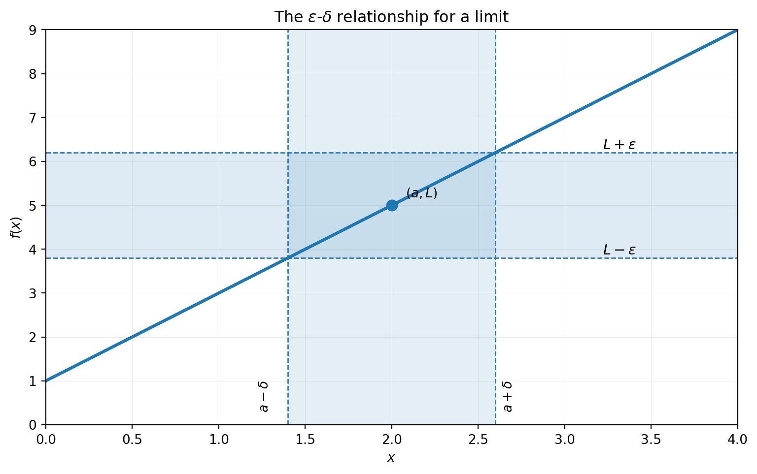
The figure should be read as a challenge-response process. A challenger chooses the output tolerance $\varepsilon$. The proof must then produce an input tolerance $\delta$ that works for every nonzero input displacement smaller than $\delta$. Choosing one convenient tolerance is not enough; the rule must respond to every positive $\varepsilon$.

The word “every” matters. Checking a few decimal inputs or one graphing window can support a conjecture, but it cannot establish the promise for every requested output tolerance. Estimating Limits from Graphs, Tables, and Formulas develops estimation; The Formal Definition of a Limit develops proof.

Three questions that look impossible without limits

The same logical structure appears in several problems that motivated calculus.

What is an instantaneous rate?

An average velocity over a nonzero interval is unambiguous:

$$v_{\mathrm{avg}} =\frac{s(t+h)-s(t)}h.$$

Instantaneous velocity cannot be obtained by substituting $h=0$, because that would divide by zero. Instead, the interval remains nonzero while its length tends to zero. If the average velocities approach one finite value, that value defines the derivative. The limit does not pretend the interval has zero duration; it identifies the stable rate revealed by every sufficiently short interval.

What is the area under a curved boundary?

A finite collection of rectangles gives an approximation. Increasing the number of rectangles usually improves it, but no particular finite mesh is the curved region itself. An integral asks whether all sufficiently fine partitions force their sums toward one value. Again, exactness comes from control of the refinement process rather than from completing infinitely many physical steps.

What is the value of an infinite sum?

The expression

$$1+\frac12+\frac14+\frac18+\cdots$$

does not instruct us to finish infinitely many additions. It defines a sequence of finite partial sums:

$$S_n =1+\frac12+\frac14+\cdots+\frac1{2^n}.$$

If $S_n$ approaches $2$, the series is assigned the sum $2$. The claim is about the limit of finite objects. Limits therefore preserve ordinary arithmetic at every stage while defining what the refining sequence approaches.

These three settings—rates, accumulated quantities, and series—look different, but each replaces an impossible final operation with a controlled limiting statement.

Direction matters

Approaching a point from the left and from the right are different processes. The number-line figure below makes the direction explicit. Inputs on either side can move toward $a$ without ever equaling $a$.

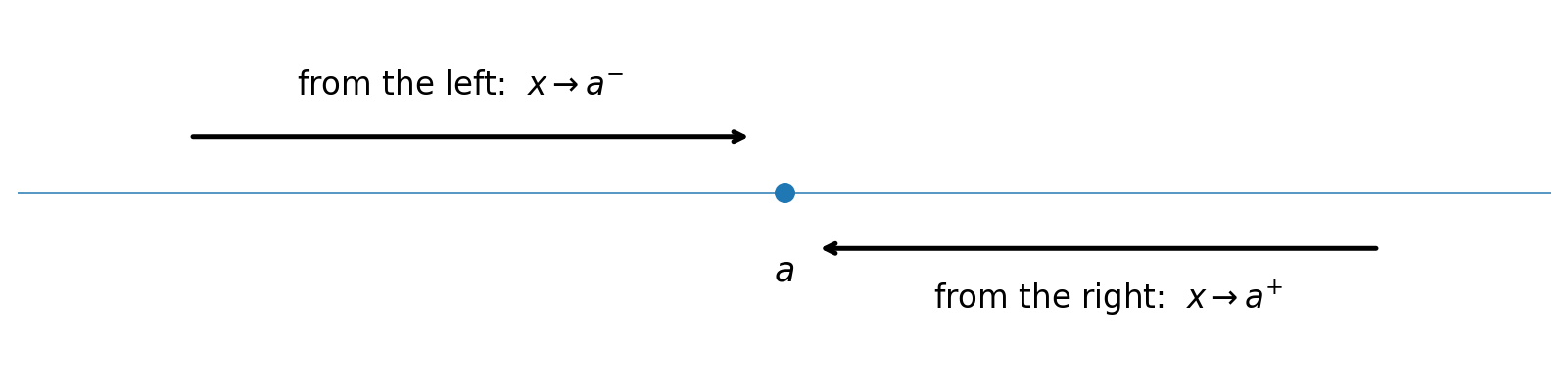
The two-sided limit exists only if the left-hand and right-hand limits both exist and equal the same value. For

$$q(x)=\frac{|x|}{x},$$

the left-hand outputs remain $-1$, while the right-hand outputs remain $1$. No single number describes both sides. Writing merely “the limit does not exist” is incomplete reasoning; the incompatible one-sided limits explain why.

Direction also matters at a domain endpoint. The real-valued function $\sqrt{x}$ has no domain points to the left of zero. Its limit at the endpoint is therefore understood from within its domain:

$$\lim_{x\to0^+}\sqrt{x}=0.$$

This is not a weakened version of a two-sided limit. It is the appropriate statement for the available inputs.

Numerical evidence, graphical evidence, and analytic reasoning

A table and a graph are valuable because they help us see what to investigate. They can suggest a limiting value, reveal a jump, or show rapid growth. Their limitations are equally important.

A numerical table samples finitely many inputs. It may miss oscillations between samples or be distorted by rounding. A graph displays finitely many pixels across a selected window. It may hide a small hole, make a steep finite slope look vertical, or make a slowly changing function appear constant. Analytic reasoning examines the function itself and can establish a result for every sufficiently close input.

Consider

$$f(x)=\frac{\sin x}{x}.$$

A calculator table near zero strongly suggests a limit of $1$, but the table does not explain why every closer input behaves consistently. A geometric comparison on the unit circle yields local inequalities that squeeze the quotient between functions with limit $1$. The proof converts a visual insight into an analytic guarantee.

The representations should cooperate rather than compete:

1. use a graph or table to form a conjecture;
2. identify a relevant algebraic, geometric, or comparison structure;
3. carry out an analytic argument;
4. return to the representation and confirm that the conclusion fits the observed behavior.

When the representations disagree, investigate the discrepancy instead of choosing the preferred answer.

A hole does not decide a limit

Consider

$$f(x)=\frac{x^2-1}{x-1}.$$

At $x=1$, the expression is undefined. But for every $x\ne1$, it simplifies to $x+1$. Therefore,

$$\lim_{x\to1}\frac{x^2-1}{x-1}=2.$$

This is not a technical curiosity. Data can be missing at one instant while nearby measurements still reveal a stable trend. Conversely, assigning a value at the missing instant does not force the surrounding trend to agree with it.

The graph below shows this separation visually. The curve approaches the open point at $(2,4)$ from both sides. The open marker records that the original formula does not define the function at $x=2$; it does not erase the nearby trend.

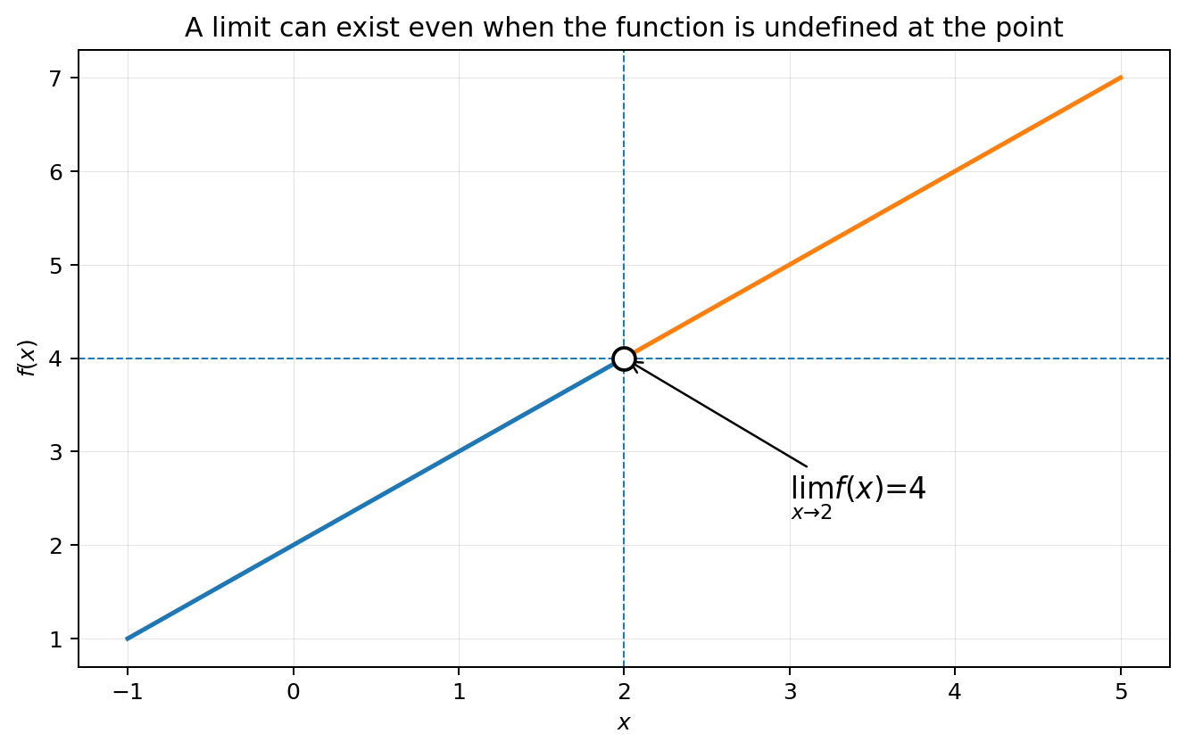
This distinction supports a useful repair. If the only defect is that $f(2)$ is missing or has the wrong value, defining $f(2)=4$ makes the function continuous there. The limit identifies the unique value that repairs the hole.

Not every undefined point is removable. For

$$r(x)=\frac1{x-2},$$

the outputs grow without bound with opposite signs on the two sides. No finite choice of $r(2)$ could change that nearby behavior. Limits therefore distinguish a missing point that can be repaired from a vertical asymptote that cannot.

Limits create the machinery of calculus

A derivative is a limit of average rates of change:

$$f'(x)=\lim_{h\to0}\frac{f(x+h)-f(x)}{h}.$$

An integral is a limit of finite sums:

$$\int_a^b f(x)\,dx =\lim_{n\to\infty} \sum_{i=1}^{n}f(x_i^*)\,\Delta x.$$

These formulas work because a limit can extract an exact value from an indefinitely refining process.

Limits also describe two kinds of infinity without turning infinity into a number. In an infinite limit, outputs grow without bound near a finite input; see Infinite Limits and Vertical Asymptotes. In a limit at infinity, the input moves outward without bound while outputs may approach a finite long-run value; see Limits at Infinity and Horizontal Asymptotes.

Infinity is a direction of behavior

The statement

$$\lim_{x\to2^+}\frac1{x-2}=+\infty$$

does not say that the function equals an object called infinity. It says that every positive output bound can be exceeded by choosing $x>2$ sufficiently close to $2$. The corresponding left-hand limit is $-\infty$. Since the signs disagree, there is no two-sided infinite limit with one sign, although $x=2$ is still a vertical asymptote.

By contrast,

$$\lim_{x\to\infty}\frac{3x+1}{x+4}=3$$

describes the far-right end of the graph. Dividing numerator and denominator by $x$ gives

$$\frac{3+\frac{1}{x}}{1+\frac{4}{x}},$$

whose reciprocal terms vanish as $x$ grows. The horizontal asymptote $y=3$ describes long-run behavior, not a barrier. The graph may cross it at finite inputs.

Keeping these roles separate prevents common statements such as “plug in infinity” or “the function reaches infinity.” Infinity signals how an input or output behaves; it is not substituted as an ordinary real number.

When algebra is not enough

Some expressions resist simplification because a bounded factor oscillates forever. Consider

$$x^2\sin(\frac{1}{x}).$$

The sine term has no limit as $x\to0$, but its magnitude never exceeds $1$. Therefore

$$|x^2\sin(\frac{1}{x})|\le x^2.$$

The right side tends to zero, forcing the product to zero. The Squeeze Theorem formalizes this transfer of limiting behavior through local bounds.

The canonical oscillation graph below shows why direct visual convergence fails for $\sin(\frac{1}{x})$. The oscillations become more rapid near zero and never settle near one output.

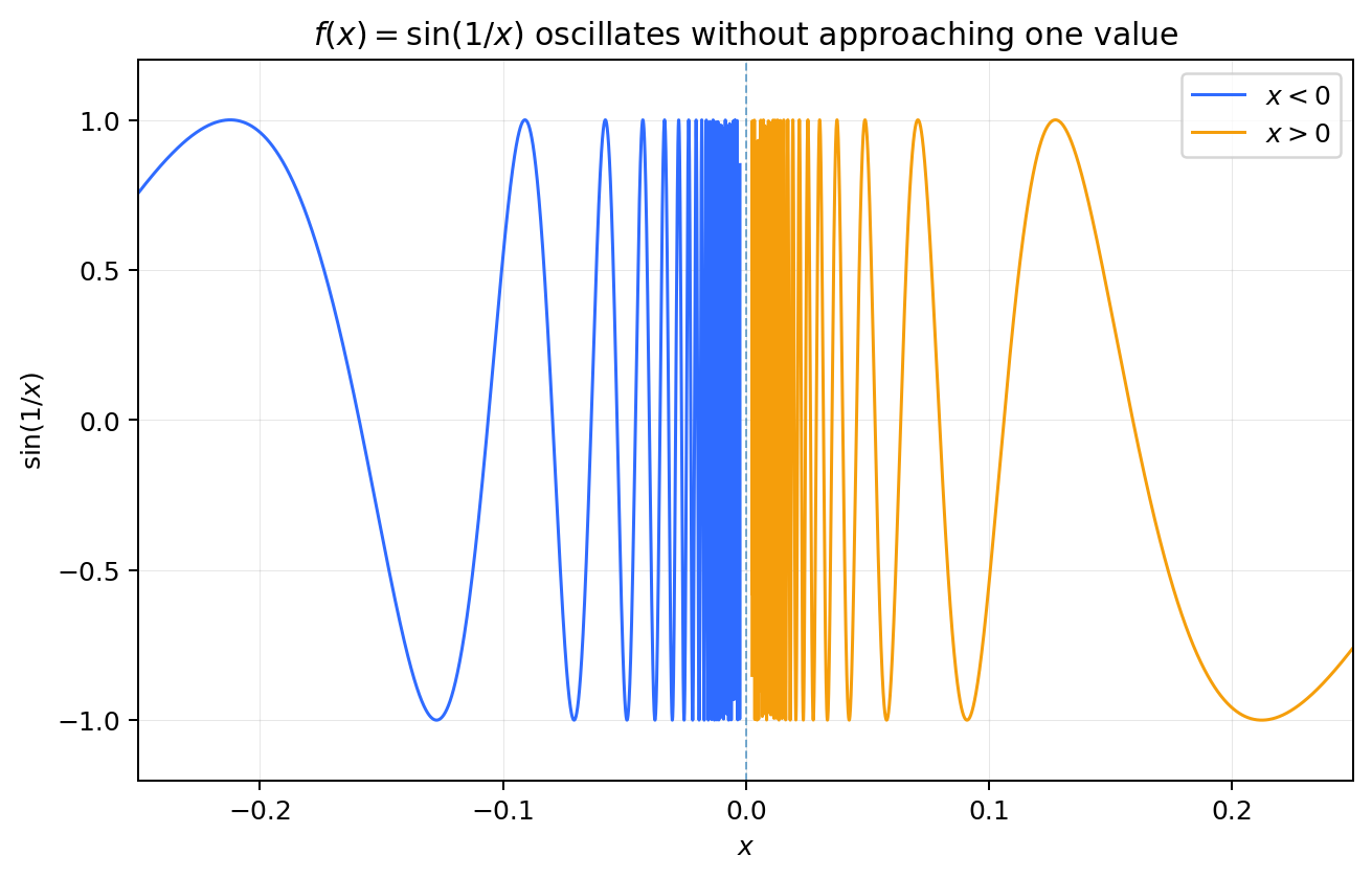
Multiplying by $x^2$ changes the conclusion because the oscillation is confined between $-x^2$ and $x^2$. The frequency may diverge, yet the amplitude collapses. This distinction appears in signal analysis and approximation theory: rapid variation does not prevent convergence when a shrinking envelope controls magnitude.

Bounds must remain local when they were derived locally. If an estimate depends on $|x-a|<1$, that restriction belongs to every later step that uses the estimate. A valid nearby bound should never be presented as a global identity.

Limits as guarantees in measurement and computation

Real measurements have finite resolution. A limit does not remove that fact; it explains what a model predicts as resolution improves. Suppose position samples are separated by $0.10\,\mathrm{s}$, then $0.01\,\mathrm{s}$, then $0.001\,\mathrm{s}$. The resulting average velocities may stabilize, but measurement noise can eventually dominate. The mathematical derivative describes the limiting model, while experimental practice must also quantify uncertainty and instrument response.

Numerical algorithms use the same separation. A finite computation returns an approximation. A convergence theorem explains whether refining the computation drives the approximation toward a well-defined result. Without convergence, producing more digits can create false confidence rather than accuracy.

For example, the bisection method starts with a continuous function whose endpoint values have opposite signs. Each step halves the interval while preserving a root inside. After $n$ steps, the interval width is

$$\frac{b-a}{2^n}.$$

The finite interval supplies an explicit error bound, and the limiting process explains why the approximations converge. Continuity provides the existence guarantee; the algorithm provides controlled localization.

A thought experiment about altered point values

Suppose two functions agree at every input except $x=a$. Must they have the same limit as $x\to a$? Yes, whenever either limit exists. The punctured-neighborhood definition excludes the point itself, so changing one isolated value cannot change the limit.

Now alter the function at infinitely many points approaching $a$. The conclusion can change. If the altered points carry outputs far from the proposed limit no matter how close they lie to $a$, the output-control promise fails. This contrast shows that limits ignore the target point but do not ignore arbitrary nearby behavior.

The same reasoning explains why a graph is not merely “mostly close” to its limit. Every sufficiently close domain point must satisfy the requested tolerance, except the target input itself. Rare but recurring spikes can destroy a limit.

Why the definition is designed backward

When proving a limit, we often begin with the desired output condition and work backward to find a sufficient input condition. For

$$\lim_{x\to2}(3x+1)=7,$$

the output difference is

$$|(3x+1)-7|=3|x-2|.$$

To make this smaller than $\varepsilon$, it is sufficient to require

$$|x-2|<\frac{\varepsilon}{3}.$$

That backward design suggests $\delta=\frac{\varepsilon}{3}$. The formal proof then runs forward: assume $0<|x-2|<\delta$ and verify that the output difference is smaller than $\varepsilon$. Discovery and verification move in opposite directions, and keeping them distinct makes proofs easier to construct and read.

Limits preserve structure—but only under hypotheses

Limit laws allow sums, products, and quotients to be handled from the limits of their parts. They are not permission to manipulate undefined expressions as ordinary numbers. If $f(x)\to L$ and $g(x)\to M$, then the sum approaches $L+M$ and the product approaches $LM$. For a quotient, the conclusion additionally requires $M\ne0$.

When numerator and denominator both tend to zero, the expression has the indeterminate form $\frac{0}{0}$. That phrase does not name a value. It warns that the separate limits do not determine the quotient limit. Compare

$$\frac{x}{x}=1, \qquad \frac{x^2}{x}=x, \qquad \frac{x}{x^2}=\frac1x.$$

As $x\to0$, every unsimplified numerator and denominator tends to zero, but the quotient behaviors are $1$, $0$, and unbounded. Factoring, rationalization, identities, comparison, or later derivative-based methods are needed to reveal the actual behavior.

The topology hidden in ordinary language

Phrases such as “near,” “eventually,” and “arbitrarily close” express a general pattern. A limit ignores finitely many early stages and focuses on behavior after a process enters every requested neighborhood. In a sequence, “sufficiently large $n$” plays the role that “sufficiently close $x$” plays for a function.

This shared structure lets the same idea organize continuous change, discrete sequences, infinite series, numerical algorithms, and approximating families of functions. Introductory calculus already contains the essential bargain: specify the output control required, then prove that an input or refinement condition guarantees it.

That is why limits matter beyond any one formula. They turn approximation into exact mathematics without confusing an unending process with a completed physical action.

A final comparison: approaching versus attaining

A sequence can approach a value without ever containing it. The finite sums

$$1, \quad 1+\frac12, \quad 1+\frac12+\frac14, \quad\ldots$$

remain below $2$, yet their limit is $2$. A function can also attain its limiting value repeatedly, cross it, or avoid it entirely. None of those possibilities alone determines the limit.

What matters is eventual control: after inputs are restricted sufficiently close to the target—or indices are taken sufficiently large—every remaining output must lie inside the requested tolerance. This criterion is stricter than visual resemblance and more flexible than requiring equality.

The distinction explains why asymptotes may be crossed, why holes may have limits, and why an infinite series may have a finite sum. “Approaches” is not an informal substitute for “almost equals.” It describes a quantified relationship that remains reliable under every finer demand.

Once that relationship is established, calculus can use it as a foundation. Continuity aligns the limit with an actual value. Differentiation applies a limit to shrinking rates. Integration applies a limit to refining sums. The later concepts differ in purpose, but the logical engine is the same.

The larger idea

Limits are a bridge between the finite and the infinite. They do not ask us to complete infinitely many steps. They ask whether the pattern of those steps determines one unavoidable destination.

Prove a limit from the definition

To prove $\lim_{x\to2}(3x+1)=7$, note $|(3x+1)-7|=3|x-2|$. Given $\varepsilon>0$, choose $\delta=\frac{\varepsilon}{3}$. Then $0<|x-2|<\delta$ forces the output error below $\varepsilon$. We work backward to design $\delta$, then forward to verify it.

Check your understanding

Before moving on, test whether you can separate evidence from conclusion. A table may strongly suggest a limit, and a graph may make the same behavior visible, but neither by itself proves what happens at every sufficiently close input. Algebra can sometimes supply that proof by replacing an indeterminate expression with an equivalent one on a punctured neighborhood. The formal definition goes further: it turns “as close as desired” into a guarantee that survives every requested output tolerance.

Also ask which feature of the problem the limit is describing. Is the input approaching a finite point, moving without bound, or approaching from only one side? Is the output settling near a number, increasing without bound, or oscillating? Naming both the input behavior and output behavior prevents several common errors. In particular, infinity is not a number substituted into a formula, and an undefined function value does not automatically destroy a nearby limit. These distinctions are the conceptual grammar on which the rest of calculus depends.

Can a limit exist where the function is undefined?

Show the reasoning

Yes. The condition $0<|x-a|$ excludes the point, so a removable hole does not determine nearby behavior.

Pathways into the Lessons

• Begin with Estimating Limits from Graphs, Tables, and Formulas to coordinate numerical, graphical, and analytic evidence.
• Continue through One-Sided Limits and the Existence of a Limit before studying discontinuities or asymptotes.
• Use Limit Laws and Algebraic Techniques for rigorous calculation and The Squeeze Theorem when comparison is more useful than simplification.
• Move to Continuity at a Point and Derivative as a Limit once nearby behavior is secure.

Sources

• OpenStax Calculus, Volume 1, chapters on limits, continuity, and derivatives.
• AP Calculus AB course overview, for the intended curriculum sequence.