Limits at Infinity and Horizontal Asymptotes

A limit at infinity describes what function outputs approach while inputs move without bound. The input does not arrive at an object called infinity, because infinity is not a real number. Instead, the analysis follows the graph farther and farther to the right or left. A finite end limit creates a horizontal asymptote on the corresponding end. This lesson develops graphical, algebraic, and formal ways to justify that long-run behavior.

Move outward rather than toward a finite point

In a finite-point limit such as $\lim_{x\to a}f(x)$, inputs approach the real number $a$. In a limit at infinity, inputs move outward without bound. The notation $x\to\infty$ means that $x$ becomes larger than every fixed positive threshold under consideration. The notation $x\to-\infty$ means that $x$ becomes more negative than every fixed threshold. Neither notation substitutes infinity into the function.

The right-end statement $\lim_{x\to\infty}f(x)=L$ says outputs can be made arbitrarily close to finite number $L$ by taking $x$ sufficiently large. The left-end statement $\lim_{x\to-\infty}f(x)=L$ says the same for sufficiently negative inputs. The two limits can agree or differ. Each end of a graph must be studied independently. Symmetry can sometimes relate them but should not be assumed.

Limits at infinity describe remote behavior rather than every finite input. A function can oscillate, cross a candidate asymptote, or contain local irregularities before eventually settling near its limiting value. The phrase “eventually” is central. Long-run control begins beyond some threshold. It does not erase what happened earlier.

Interpret a horizontal asymptote

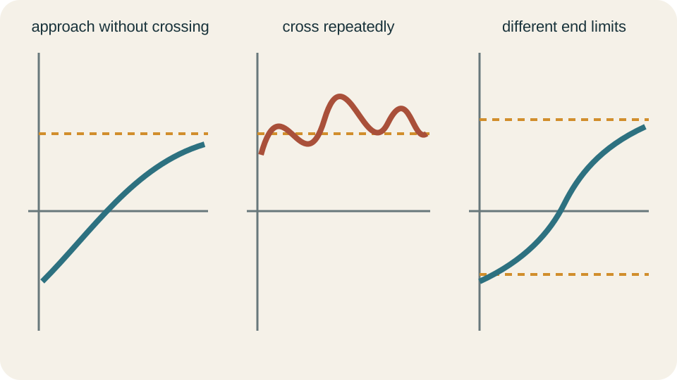
If $\lim_{x\to\infty}f(x)=L$ or $\lim_{x\to-\infty}f(x)=L$, then $y=L$ is a horizontal asymptote on that end. The horizontal line records the finite output approached remotely. A function can have one horizontal asymptote shared by both ends. It can also have different asymptotes on its left and right ends. The definition is end-specific.

A horizontal asymptote is not a barrier. The function $f(x)=1+\dfrac{\sin x}{x}$ approaches one as $x\to\infty$ and crosses $y=1$ whenever $\sin x=0$ for positive $x$. The oscillations shrink because $|\sin x/x|\leq1/x$. Crossing does not contradict approach. The asymptote constrains distance from the line for sufficiently large input.

The function need not ever equal its asymptote. For $f(x)=1+1/x^2$, every nonzero finite input produces a value above one. Yet $1/x^2$ approaches zero, so $f(x)$ approaches one on both ends. Equality at a finite point is irrelevant to the end limit. Approach describes arbitrary closeness, not eventual identity.

State the formal right-end definition

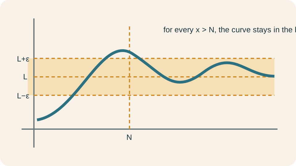
The formal statement $\lim_{x\to\infty}f(x)=L$ uses an output tolerance and an input threshold. For every $\varepsilon>0$, there must exist a number $N$ such that $x>N$ implies $|f(x)-L|<\varepsilon$. The Greek letter epsilon, $\varepsilon$, represents any requested positive output distance. The number $N$ is a sufficiently large input threshold. It need not be an integer.

The absolute-value inequality $|f(x)-L|<\varepsilon$ means the output lies inside the horizontal band $L-\varepsilon<f(x)<L+\varepsilon$. The threshold requirement says all inputs to the right of $N$ must produce outputs inside that band. One isolated successful point is insufficient. The entire tail of the graph must remain close. Smaller tolerances may require larger thresholds.

The order of the statement matters. A challenger chooses any positive tolerance first. The proof then supplies a threshold that works for every larger input. The threshold may depend on the tolerance. A single finite threshold rarely works for every arbitrarily small tolerance. This structure turns visual approach into a precise guarantee.

State the formal left-end definition

The statement $\lim_{x\to-\infty}f(x)=L$ requires that for every $\varepsilon>0$, there exists $N>0$ such that $x<-N$ implies $|f(x)-L|<\varepsilon$. The positive number $N$ controls how far left the input must lie. Using $x<-N$ makes the threshold direction explicit. Larger $N$ means a farther-left tail. The output band is unchanged.

For $f(x)=1/x$, both end limits equal zero. Given $\varepsilon>0$, choose $N>1/\varepsilon$. If $x>N$ or $x<-N$, then $|x|>N$. Therefore $|1/x|<1/N<\varepsilon$. The same absolute-value estimate handles both ends.

Signs still matter for the direction of approach. As $x\to\infty$, $1/x$ approaches zero through positive values. As $x\to-\infty$, it approaches through negative values. The limit value is the same. A graph or one-sided sign description can preserve this additional information.

Use reciprocal-power limits

For every positive integer $p$, $1/x^p\to0$ as $x\to\infty$ and as $x\to-\infty$. The exponent $p$ controls the rate and sign behavior. Even powers remain positive on both ends. Odd powers are negative on the left and positive on the right. Their magnitudes still approach zero.

Constants multiply these limits predictably. If $c$ is fixed, then $c/x^p\to0$. Finite sums of reciprocal powers also approach zero by limit laws. These facts support rational-function normalization. Lower-degree terms become reciprocal corrections after division by a dominant power.

The notation $1/x^p\to0$ is a limit statement, not an equality for finite $x$. The fraction never becomes zero when its numerator is one. It can be made smaller in magnitude than any positive tolerance. This distinction mirrors asymptotic approach generally. Calculus turns “negligible in the long run” into a precise limit.

Identify dominant polynomial terms

For polynomial $P(x)=a_nx^n+a_{n-1}x^{n-1}+\cdots+a_0$, the highest-power nonzero term dominates magnitude as $|x|$ grows. Factor $x^n$ to write $P(x)=x^n\left(a_n+\dfrac{a_{n-1}}{x}+\cdots+\dfrac{a_0}{x^n}\right)$. The reciprocal terms approach zero. The bracket approaches leading coefficient $a_n$. End behavior is therefore governed by $a_nx^n$.

Degree parity and leading-coefficient sign determine polynomial ends. An even power has the same sign on both ends, while an odd power changes sign. A positive even leading term rises on both ends. A negative even leading term falls on both ends. Odd-degree ends point in opposite vertical directions.

This dominant-term reasoning is not permission to erase lower terms at finite inputs. Near zeros or moderate values, lower-degree terms can matter greatly. Dominance is an asymptotic comparison. Factoring and limits justify when the relative corrections vanish. The method explains rather than merely labels end behavior.

Normalize rational functions

A rational function is a quotient $R(x)=P(x)/Q(x)$ of polynomials where $Q(x)\neq0$. To study end behavior, divide every numerator and denominator term by a suitable highest power of $x$. Dividing by the denominator’s degree exposes whether the numerator grows slower, equally fast, or faster. Reciprocal terms then approach zero. The resulting limit follows from ordinary limit laws when the denominator limit is nonzero.

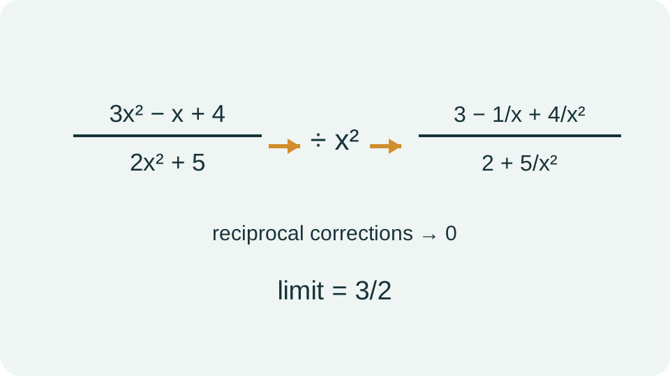
Consider $\dfrac{3x^2-x+4}{2x^2+5}$. Dividing every term by $x^2$ gives $\dfrac{3-\dfrac{1}{x}+\dfrac{4}{x^2}}{2+\dfrac{5}{x^2}}$. Every reciprocal-power term approaches zero. The limit is therefore $\dfrac{3}{2}$ on both ends. The horizontal asymptote is $y=\dfrac{3}{2}$.

Normalization preserves equality for every nonzero $x$. It does not substitute infinity. It rewrites the function into a constant leading structure plus terms whose limits are known. This algebraic chain is the justification behind degree comparisons. A degree slogan without normalization hides the reason.

Compare rational-function degrees

If numerator degree is less than denominator degree, normalization makes every numerator term approach zero while the denominator approaches a nonzero leading coefficient. The limit is zero. Thus $y=0$ is a horizontal asymptote on both ends for such polynomial quotients. The conclusion assumes real inputs where the function is defined. Finite vertical asymptotes do not alter the remote limit.

If the degrees are equal, the limit is the ratio of leading coefficients. For $\dfrac{5x^3-2x}{-x^3+7x^2+1}$, divide by $x^3$. The normalized expression is $\dfrac{5-\dfrac{2}{x^2}}{-1+\dfrac{7}{x}+\dfrac{1}{x^3}}$. Reciprocal terms vanish, leaving $-5$. Both end limits equal negative five.

If numerator degree exceeds denominator degree, no finite horizontal limit follows from leading-degree comparison. The quotient may grow without bound or approach a slant or higher-degree polynomial asymptote after division. “No horizontal asymptote” does not mean “no asymptotic structure.” Polynomial long division reveals the appropriate comparison. The degree difference predicts the asymptote’s polynomial degree. The remainder term must still be checked to confirm that it vanishes relative to the denominator.

Analyze a lower-degree numerator

Evaluate $\lim_{x\to\infty}\dfrac{4x-1}{x^2+3}$. Divide numerator and denominator by $x^2$. The result is $\dfrac{\dfrac{4}{x}-\dfrac{1}{x^2}}{1+\dfrac{3}{x^2}}$. The numerator approaches zero. The denominator approaches one.

The quotient limit is zero. Therefore $y=0$ is a right-end horizontal asymptote. The same normalization works as $x\to-\infty$. Odd reciprocal terms change sign, but they still approach zero. The left-end limit is also zero.

A rough growth comparison supports the result. The numerator grows like $x$, while the denominator grows like $x^2$. Their ratio behaves like $1/x$. The denominator outruns the numerator in magnitude. Formal normalization turns that intuition into calculation.

Use polynomial division for slant behavior

Consider $f(x)=\dfrac{x^2+1}{x}$. Polynomial division gives $f(x)=x+1/x$. Since $1/x\to0$, the difference $f(x)-x$ approaches zero. The line $y=x$ is a slant asymptote. There is no finite horizontal asymptote.

A slant asymptote need not be horizontal because the function and comparison line can both grow. The defining idea is that their vertical difference approaches zero. If the numerator degree exceeds denominator degree by more than one, polynomial division may produce a higher-degree polynomial asymptote. The remainder divided by the denominator must approach zero. Division separates dominant quotient from vanishing correction.

The graph can cross a slant asymptote as well. Asymptotes describe closeness at remote inputs. They are not walls. The remainder’s sign determines which side the graph occupies at a given input. If the remainder changes sign, crossings can occur.

Handle radicals with absolute values

The identity $\sqrt{x^2}=|x|$ is essential. A square root returns the nonnegative principal root. For positive $x$, $|x|=x$. For negative $x$, $|x|=-x$. Replacing $\sqrt{x^2}$ by $x$ on the left end creates a sign error.

Consider $f(x)=\dfrac{x}{\sqrt{x^2+1}}$. Factor $x^2$ inside the radical to get $\sqrt{x^2+1}=|x|\sqrt{1+1/x^2}$. Therefore $f(x)=\dfrac{x/|x|}{\sqrt{1+1/x^2}}$. The denominator approaches one. The factor $x/|x|$ determines the end sign.

As $x\to\infty$, $x/|x|=1$, so the limit is one. As $x\to-\infty$, $x/|x|=-1$, so the limit is negative one. The graph has different horizontal asymptotes on its two ends. Absolute value preserves the correct square-root sign. Treating both ends identically would erase information carried by the numerator’s sign.

Simplify even powers under radicals

Consider $f(x)=\dfrac{3x^2-x+4}{\sqrt{4x^4+1}}$. Factor $x^4$ inside the radical. This gives $\sqrt{4x^4+1}=\sqrt{x^4}\sqrt{4+1/x^4}$. Since $\sqrt{x^4}=|x^2|=x^2$, no end-dependent sign remains. The square $x^2$ is nonnegative.

Divide numerator and denominator by $x^2$. The expression becomes $\dfrac{3-1/x+4/x^2}{\sqrt{4+1/x^4}}$. Reciprocal terms approach zero. The numerator approaches three, and the denominator approaches two. Both end limits equal $3/2$.

The absolute-value step is still logically necessary even though it simplifies. Writing $\sqrt{x^4}=x^2$ is correct because $x^2\geq0$. Writing $\sqrt{x^2}=x$ is not correct for negative $x$. Checking the exponent inside the square root prevents pattern-based mistakes. The principal square root always returns a nonnegative value.

Study exponential end behavior

For base $b>1$, $b^x\to\infty$ as $x\to\infty$ and $b^x\to0$ as $x\to-\infty$. The left behavior follows from $b^x=1/b^{-x}$. Thus $y=0$ is a left-end horizontal asymptote. The function never reaches zero, but it approaches it. Exponential growth and decay swap when direction reverses.

For $0<b<1$, the end behaviors reverse. The function decays toward zero on the right and grows on the left. A vertical shift $f(x)=b^x+L$ moves the horizontal asymptote from zero to $y=L$. Multiplication changes scale but not the zero asymptote before shifting. Transformations provide a fast qualitative check.

Exponential terms dominate polynomials on the growing end. For example, $x^3/2^x\to0$ as $x\to\infty$. A proof can use later tools such as repeated L’Hôpital reasoning or established growth theorems. At this stage, graphs and known growth hierarchies provide context. Algebraic degree rules alone apply only to rational polynomial quotients.

Study logarithmic end behavior

The natural logarithm satisfies $\ln x\to\infty$ as $x\to\infty$. Its growth is unbounded but slower than every positive power of $x$. The domain requires $x>0$. Therefore a real left-end limit as $x\to-\infty$ is not defined for $\ln x$. Domain must be checked before end behavior is discussed.

For $\ln x/x$, the denominator eventually outgrows the numerator, and the limit is zero as $x\to\infty$. This statement requires a theorem or later calculus method beyond polynomial degree comparison. The function has a right-end horizontal asymptote $y=0$. It approaches from positive values for $x>1$. A graph supports but does not alone prove the result.

Logarithmic transformations can change domain and asymptotes. The function $\ln(x^2+1)$ is defined for every real $x$ and grows on both ends. The function $1/\ln x$ has a vertical issue at $x=1$ and approaches zero as $x\to\infty$. Each expression must be analyzed from its own domain and growth structure. Function family matters.

Distinguish finite and infinite end limits

A finite end limit produces a horizontal asymptote. An infinite end limit such as $\lim_{x\to\infty}f(x)=\infty$ means outputs grow beyond every fixed positive bound. It does not produce a finite horizontal asymptote. The infinity symbol describes unbounded behavior. It is not the value of the function.

For every output bound $M>0$, the statement $f(x)\to\infty$ requires a threshold $N$ such that $x>N$ implies $f(x)>M$. The capital $M$ plays the role of a requested output height. Larger requested heights may require larger input thresholds. This definition parallels finite end limits but replaces a tolerance band with a lower bound. Negative infinity uses upper bounds below $-M$.

A rational function with numerator degree one larger than denominator degree often grows approximately linearly rather than approaching a finite value. Reporting simply “the limit does not exist” loses useful direction. State whether it grows to positive infinity, negative infinity, or follows different behavior on the two ends. End behavior deserves the most informative correct description. A polynomial asymptote can provide that description even when no finite end limit exists.

Interpret long-run models cautiously

Suppose a population model satisfies $P(t)\to K$ as $t\to\infty$. The number $K$ is the model’s long-run limiting population. For any chosen tolerance, the model eventually stays within that tolerance of $K$. The statement does not require the population to equal $K$ at a finite time. It also does not prevent crossing $K$.

The conclusion is conditional on model validity. Environmental change, migration, policy, or new mechanisms can make the formula unreliable in the distant future. A mathematical limit describes the formula indefinitely. A scientific claim requires reasons that the formula remains applicable. Extrapolation should be labeled.

Units belong to the limiting value. If $Q(t)\to12.0\,\mathrm{mg}$, then the tolerance should also be expressed in milligrams. The input threshold carries time units. A statement such as “after some sufficiently large time” should identify the time scale when used quantitatively. Dimensional interpretation makes the model concrete.

Estimate end behavior numerically and graphically

A table can sample increasingly large positive and negative inputs. Stable outputs suggest a candidate limit. A graph can show whether the tails flatten near a horizontal line. Neither method alone proves the limit because finite sampling misses all later behavior. They are exploratory tools that guide algebra or proof.

Graphing windows can mislead. A slowly growing function may appear horizontal over a limited range. A function with long transient behavior may appear to approach one value before departing. Logarithmic scales or larger ranges can reveal hidden growth. Analytical structure is needed to justify the final conclusion.

Numerical subtraction can also lose precision for large inputs. Expressions equivalent algebraically may behave differently in floating-point arithmetic. Normalization often improves numerical stability by keeping values near order one. A table should use formulas and scales suited to the range. Computational evidence must be interpreted with numerical limitations.

Diagnose common limit-at-infinity errors

One error is substituting infinity as though it were a number. Instead, rewrite the function and apply limit laws. Another is looking only at leading coefficients while ignoring degree. Coefficient ratios apply directly only when numerator and denominator degrees match. Normalization exposes the correct case.

Radical errors arise from replacing $\sqrt{x^2}$ with $x$ on the negative end. The correct result is $|x|$. Another error is assuming the two ends must share one horizontal asymptote. Odd signs and asymmetric functions can produce different limits. Each end requires separate analysis.

Interpretive errors include treating an asymptote as an uncrossable wall or assuming the function eventually equals it. Both claims are stronger than the limit definition. Domain errors also matter after algebraic simplification. The original function may exclude finite points even when a simplified expression appears defined. End limits do not restore those points.

Practice a complete end-behavior routine

First identify the direction $x\to\infty$ or $x\to-\infty$ and check the domain. Second identify the function family and dominant structure. Third normalize rational expressions or factor dominant powers carefully. Fourth apply reciprocal, limit-law, and sign facts. Fifth interpret any finite result as an end-specific horizontal asymptote.

Evaluate $\lim_{x\to-\infty}\dfrac{2x^2+1}{5x^2-x}$. Divide by $x^2$ to obtain $\dfrac{2+1/x^2}{5-1/x}$. Reciprocal terms vanish on the left end. The limit is $2/5$. Equal degrees make this the leading-coefficient ratio.

For $\dfrac{x}{\sqrt{x^2+9}}$, factor $x^2$ under the radical. The expression becomes $\dfrac{x/|x|}{\sqrt{1+9/x^2}}$. Its right-end limit is one, and its left-end limit is negative one. A sign-aware algebraic step explains the two asymptotes. The graph should approach $y=1$ on the right and $y=-1$ on the left.

Consolidate limits at infinity

Limits at infinity study outputs while inputs move without bound. A finite end limit defines a horizontal asymptote for that end. Formal definitions use output tolerances and input thresholds. Graphs may cross asymptotes because asymptotes describe remote closeness rather than barriers. The two ends can behave differently.

Rational-function end behavior follows from dominant-power normalization. Lower-degree reciprocal corrections vanish. Equal degrees yield the ratio of leading coefficients, while a lower numerator degree yields zero. Higher numerator degree calls for polynomial division or unbounded analysis. Radical normalization requires absolute-value awareness.

A strong solution does not substitute infinity. It checks domain, direction, degree, sign, and units. It distinguishes finite limits from infinite growth and mathematical formulas from indefinitely valid physical models. Graphs and tables suggest behavior, while algebra and definitions justify it. End behavior connects local limit skills with global function structure.