Infinite Limits and Vertical Asymptotes

An infinite limit describes function values that grow without bound as inputs approach a finite target. The infinity symbol does not name a real-number output, and the function never needs to equal infinity. One-sided analysis is essential because signs can differ on opposite sides of the same input. Vertical asymptotes arise from this nearby unbounded behavior, not merely from an undefined function value. This lesson builds a reliable sign-analysis method and distinguishes asymptotes from holes, ordinary discontinuities, and end behavior.

Learning objectives and the central distinction

By the end of this lesson, you will interpret positive and negative infinite-limit notation. You will analyze magnitude and sign independently on each side of a candidate input. You will identify vertical asymptotes from one-sided limits. You will distinguish a removable discontinuity from a surviving denominator factor. You will also explain infinite-limit statements using arbitrary bounds and sufficiently close inputs.

Two uses of infinity appear in calculus and must remain distinct. In an infinite limit near $x=a$, the input approaches the finite number $a$ while the output grows without bound. In a limit at infinity, the input itself grows without bound. The first behavior can create a vertical asymptote, while the second can create a horizontal asymptote. The direction of the arrow notation reveals which role infinity plays.

One-sided superscripts describe the input side. The notation $x\to a^+$ means values greater than $a$ approach $a$, while $x\to a^-$ means values less than $a$ approach $a$. The signs attached to infinity describe output direction. These two sign systems answer different questions. The orientation diagram below separates them visually.

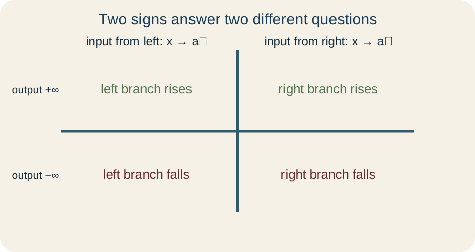
Interpret infinity as behavior, not a value

The statement $\lim_{x\to a^+}f(x)=+\infty$ says outputs exceed every chosen positive bound when allowed inputs are sufficiently close to $a$ from the right. It does not say $f(a)=\infty$. Infinity is not a real number inserted into the function. The function may be undefined at $a$, defined there, or assigned any finite value. Nearby behavior determines the limit.

Similarly, $\lim_{x\to a^-}f(x)=-\infty$ says outputs become more negative than every chosen negative threshold as inputs approach from the left. The phrase “decreases without bound” refers to ordered values, not magnitude alone. A value of negative one thousand is less than negative ten. The absolute magnitude grows while the signed output falls. Language should preserve both facts.

Arithmetic with infinity symbols is shorthand for limit behavior, not ordinary number arithmetic. Expressions such as positive constant divided by a small positive number suggest positive unbounded growth. They are reasoning cues rather than substitutions. One must still identify the sign and magnitude of every relevant factor. Treating infinity as a calculator value conceals these conditions.

State the threshold definition

The precise statement $\lim_{x\to a^+}f(x)=+\infty$ means that for every $M>0$, there exists $\delta>0$ such that $a<x<a+\delta$ implies $f(x)>M$. The letter $M$ represents an arbitrarily high positive output threshold. The letter $\delta$ represents a sufficiently small input distance. Both quantities are positive. The implication connects closeness in input to largeness in output.

For a left-hand positive infinite limit, the input condition becomes $a-\delta<x<a$. For a negative infinite limit, require $f(x)<-M$. The same positive $M$ measures how far below zero the output must fall. The definition does not ask for one universal $delta$ that handles every threshold. A more demanding threshold may require a smaller neighborhood.

This formulation explains “arbitrarily large” and “sufficiently close.” Given any height, however large, the function eventually lies above it on the stated side. A graph window showing large values is suggestive but finite. The definition makes a claim beyond every finite viewing scale. No single numerical table can exhaust all thresholds. Algebra or a theorem is needed to justify that universal behavior.

Define vertical asymptotes from one-sided limits

The line $x=a$ is a vertical asymptote when at least one one-sided limit as $x\to a$ equals $+\infty$ or $-\infty$. Only one side needs to be unbounded. The other side may have different unbounded behavior, a finite limit, or no limit. The line is vertical because its equation fixes an input rather than an output. It describes graph behavior near that input.

A function value at $a$ cannot remove the asymptote. Defining $f(a)=7$ adds one isolated point but leaves all punctured-neighborhood values unchanged. Conversely, being undefined at $a$ does not guarantee an asymptote. A hole has an undefined point with a finite nearby limit. Classification comes from limits, not domain status alone.

The graph may cross a vertical-asymptote line elsewhere only if the line equation permits another input, which it does not. No point with input $a$ belongs to the original rational function when its denominator is zero. A separately defined value can lie on that line while the asymptote remains. The term asymptote describes nearby trend, not a physical barrier. Isolated definitions and limiting behavior coexist.

Analyze magnitude and sign separately

Unbounded magnitude usually comes from a denominator approaching zero while a numerator approaches a nonzero value. Sign determines whether the output tends to positive or negative infinity. Analyze these questions separately. First confirm that magnitude grows without bound. Then determine the sign on each side.

For $f(x)=\frac{1}{x-3}$, the numerator is positive and fixed. As $x\to3^+$, the denominator is small and positive, so the quotient tends to $+\infty$. As $x\to3^-$, the denominator is small and negative, so the quotient tends to $-\infty$. The magnitude grows on both sides. Thus $x=3$ is a vertical asymptote with opposite one-sided directions.

Do not substitute vague labels such as “almost zero” without a sign. A small positive denominator and a small negative denominator produce opposite quotient signs when the numerator sign stays fixed. Test inputs such as $3.1$ and $2.9$ can support the sign analysis. Factor signs provide the general proof. The diagram below pairs a local sign chart with the two graph branches.

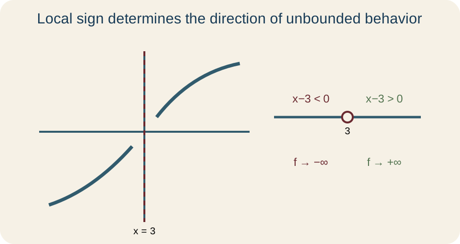
Use factor multiplicity to predict sign changes

The function $\frac{1}{(x-3)^2}$ has a denominator that is positive on both sides of three. Its magnitude approaches zero in the denominator and therefore grows without bound in the quotient. Both one-sided limits equal $+\infty$. The even exponent prevents the factor from changing sign. The graph rises on both sides.

An odd power of $x-a$ changes sign across $a$, while an even power does not. This parity pattern is useful when all other nearby factors keep fixed signs. It is not a complete rule by itself. A negative numerator reverses both output signs. Additional factors must be included in the local sign product.

For $g(x)=\frac{x-1}{(x+2)^2}$ near negative two, the numerator remains negative. The squared denominator remains positive and approaches zero. Therefore both one-sided limits equal $-\infty$. The quotient magnitude becomes unbounded. The even denominator multiplicity makes the sides agree, while the numerator determines their shared negative sign.

Simplify before declaring an asymptote

A zero denominator is a candidate signal, not a conclusion. Factor numerator and denominator first. Cancel common factors only while preserving original restrictions. Then inspect what remains. Complete cancellation can produce a hole with a finite limit.

Consider $\frac{x^2-4}{x-2}$. Factoring gives $\frac{(x-2)(x+2)}{x-2}=x+2$ for $x\ne2$. The nearby limit is four. Therefore the graph has a removable discontinuity at $(2,4)$, not a vertical asymptote. The original function remains undefined at two.

Cancellation may leave another copy of the factor. For $\frac{x^2-1}{(x-1)^2(x+2)}$, canceling one $x-1$ leaves $\frac{x+1}{(x-1)(x+2)}$. A denominator factor still approaches zero at one. The numerator and $x+2$ stay positive nearby, so $x-1$ controls sign. The result is still a vertical asymptote.

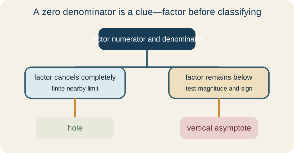
Build a systematic local sign chart

Start by factoring the expression completely. Mark zeros and excluded inputs. Choose a small interval on each side of the candidate containing no other critical points. Determine the sign of every factor in each interval. Multiply the signs to obtain the quotient’s sign.

Magnitude and sign should be recorded in separate columns. A denominator factor approaching zero explains unbounded magnitude only if the remaining numerator tends to a nonzero value. The sign chart then assigns positive or negative direction. This separation prevents a sign computation from being mistaken for a proof of divergence. It also exposes cancellations that remove unboundedness.

For $f(x)=\frac{x+1}{(x-2)(x+4)}$ near two, $x+1$ and $x+4$ are positive. The factor $x-2$ is negative on the left and positive on the right. Thus the left limit is $-\infty$ and the right limit is $+\infty$. The surviving denominator factor guarantees unbounded magnitude. State both limits before naming the asymptote.

Distinguish two-sided infinite notation

If both one-sided limits equal $+\infty$, one may write $\lim_{x\to a}f(x)=+\infty$. If both equal $-\infty$, the analogous negative statement is valid. The notation records shared unbounded direction. It is not a finite two-sided limit. The function values do not approach a real number. Some texts say the limit “diverges to infinity.”

If one side tends to $+\infty$ and the other to $-\infty$, do not write one two-sided infinite limit. The one-sided behaviors disagree. The ordinary two-sided limit does not exist. The line can still be a vertical asymptote. Asymptote classification requires only one unbounded side, whereas two-sided notation requires agreement.

If one side approaches a finite number and the other grows without bound, the two-sided limit also does not exist. Report each side separately. A piecewise function can show this mixed behavior. The vertical asymptote remains because one side is unbounded. Precise one-sided statements contain the full information.

Compare infinite limits with large finite values

A large function value does not by itself prove an infinite limit. A graph can peak at one million and remain bounded. Infinite-limit notation requires exceeding every finite threshold sufficiently close to the target. Numerical tables can suggest this pattern but sample only finitely many inputs. Algebraic structure supplies stronger evidence.

Likewise, an infinite limit does not mean every nearby value is enormous at an ordinary scale. The definition responds to any chosen threshold by allowing the neighborhood to shrink. For a very high threshold, inputs may need to be extremely close. Outside that neighborhood, values can be moderate. Locality and unboundedness work together.

Graphing technology may clip branches at the window boundary. A clipped curve can look as if it stops or reaches a highest point. Adjusting the vertical scale reveals more behavior but still cannot prove unboundedness. Use the graph as evidence to interpret a result derived from limits. Do not let display settings define the mathematics.

Connect asymptotes to domains and graphs

Rational functions are undefined where their denominators are zero before cancellation. Those inputs divide the real line into domain intervals. A vertical asymptote often separates branches whose signs and trends differ. A hole may occur within an otherwise continuous branch. Both features originate from domain restrictions but have different limits.

Logarithmic and trigonometric functions can also have vertical asymptotes. The natural logarithm tends to $-\infty$ as its positive input approaches zero. Tangent has vertical asymptotes where cosine is zero. The definition remains one-sided unbounded behavior. Denominator factoring is only one analysis method, not the definition.

The equation of a vertical asymptote is written $x=a$. A horizontal asymptote is written $y=L$ and concerns behavior as input tends to positive or negative infinity. A function may have both types. Do not interchange their equations. The input-output roles determine orientation.

Use comparison and reciprocal reasoning

Known reciprocal behavior can simplify analysis. If $u(x)\to0^+$, then $\frac{1}{u(x)}\to+\infty$. If $u(x)\to0^-$, then its reciprocal tends to $-\infty$. A nonzero numerator limit scales and possibly reverses this direction. State the sign of that numerator limit.

For $\frac{5}{(x-a)^4}$, the fourth power is positive and approaches zero on both sides. The positive numerator preserves sign. Both limits equal $+\infty$. Replacing five with negative five makes both limits $-\infty$. The exponent controls side agreement, and the numerator controls shared orientation.

Comparison can prove magnitude growth. Near zero, if $0<|u(x)|<\frac{1}{M}$, then $\frac{1}{|u(x)|}>M$. This inequality links small denominator magnitude to large reciprocal magnitude. Sign analysis then restores the signed conclusion. The reasoning mirrors the formal threshold definition.

Diagnose common mistakes

Writing $f(a)=\infty$ confuses function value with limit behavior. Declaring every denominator zero an asymptote ignores cancellation. Ignoring one-sided signs loses essential information. Writing one two-sided infinite limit for opposite sides is incorrect. Each mistake collapses distinct concepts.

Do not cancel terms across addition. Cancel only common factors. Preserve the original excluded input after valid cancellation. Restrict sign charts to a neighborhood with no other zeros or poles. A distant sign change is irrelevant to the local limit.

Do not infer unboundedness from a graph window alone. Do not treat $+\infty$ and $-\infty$ as ordinary finite outputs. Do not assume even and odd multiplicity settle sign without checking remaining factors. Check the original domain after every simplification. A dependable workflow uses simplification, magnitude analysis, local signs, one-sided notation, and classification in that order.

Guided practice and connection forward

Analyze $g(x)=\frac{-2}{(x+1)^3}$ at negative one. On the left, the cubed denominator is negative, so the quotient is positive and tends to $+\infty$. On the right, the denominator is positive, so the quotient tends to $-\infty$. Therefore $x=-1$ is a vertical asymptote. The one-sided directions disagree.

Analyze $h(x)=\frac{3}{(x-5)^2}$ at five. The squared denominator is positive on both sides and approaches zero. The positive numerator preserves a positive quotient. Both one-sided limits equal $+\infty$. Thus the two-sided infinite-limit notation is valid and $x=5$ is a vertical asymptote.

For independent synthesis, classify $\frac{x^2-4}{x-2}$ at two and explain every factoring, restriction, and limit step. Then state in threshold language what $\lim_{x\to2^-}f(x)=-\infty$ means. Finally, explain why defining $f(2)=7$ cannot change that limit. Compare the isolated value with the punctured neighborhood explicitly. Limits at infinity will next move unboundedness from the output role to the input role and connect it with horizontal asymptotes.