The Squeeze Theorem

Some functions are difficult to evaluate near a point because they oscillate, contain complicated geometry, or resist direct algebraic simplification. The Squeeze Theorem replaces direct evaluation with comparison. If a target function stays between two functions that approach the same number, the target has no other limiting value available. The theorem is simple to state but depends on careful inequality construction. This lesson develops the logic, proof, and design habits that make squeezing reliable.

Learning objectives

By the end of the lesson, you should be able to state every hypothesis of the Squeeze Theorem. You should explain what a punctured neighborhood means and why the inequalities need only hold locally. You should construct upper and lower bounds for oscillatory and absolute-value expressions. You should preserve or reverse inequality directions correctly during algebra. Every conclusion should name the common outer limit.

You will connect the geometric trapping picture with an epsilon-delta argument. You will derive the foundational limit $\lim_{x\to0}\frac{\sin x}{x}=1$ from unit-circle geometry. You will use shrinking factors to control bounded oscillation. You will also analyze one-sided, infinite, and sequence versions of the theorem. These applications show that squeezing is a proof strategy rather than one isolated formula.

Keep three tasks separate throughout the lesson. First establish an inequality valid near the point. Next calculate the two outer limits independently. Finally verify that those limits agree before transferring the conclusion. Skipping any task turns a persuasive picture into an incomplete argument.

The geometric trapping idea

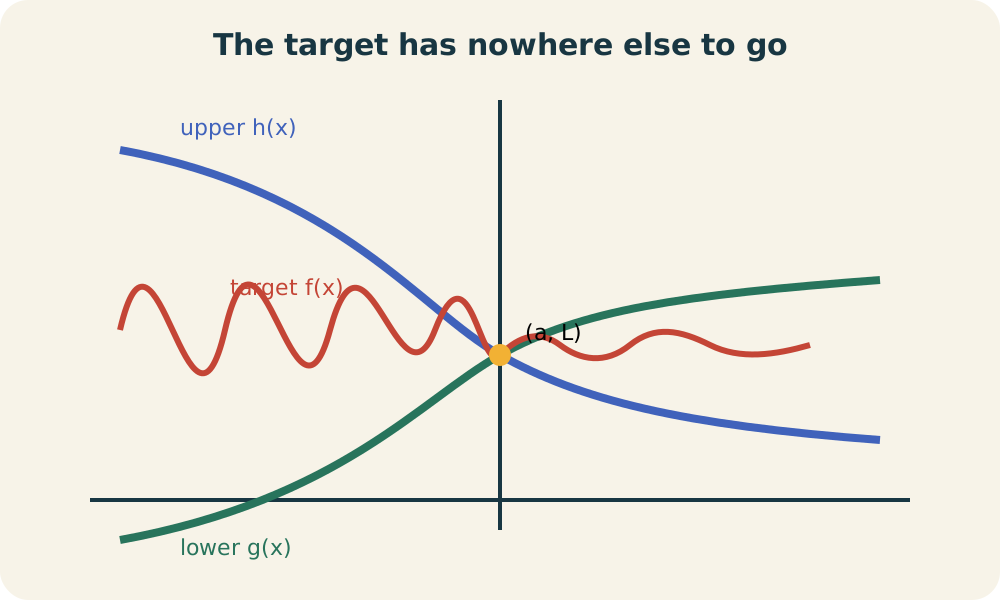
Imagine a moving point trapped vertically between two barriers. The lower barrier rises toward height $L$, and the upper barrier falls toward the same height. The trapped point may wiggle or behave irregularly. As the gap collapses, it has no room to approach a different height. This is the geometric heart of the theorem.

The picture is local rather than global. The target function can behave wildly far from the point of interest. The inequalities need only become valid sufficiently close to the input $a$. The target need not be defined at $a$. Limits describe nearby behavior rather than necessarily the value at the point.

The outer barriers must converge to the same value. If the lower function approaches $1$ and the upper approaches $3$, the target may approach any value in between or fail to approach anything. The inequalities still provide useful bounds. They do not determine a unique limit. Shared destination is the essential squeezing condition.

Precise statement of the theorem

Suppose $g(x)\le f(x)\le h(x)$ whenever $x$ lies sufficiently close to $a$ but is not equal to $a$. Suppose also that $\lim_{x\to a}g(x)=L$ and $\lim_{x\to a}h(x)=L$. Then $\lim_{x\to a}f(x)=L$. The function $f$ is the target. The functions $g$ and $h$ are lower and upper bounds.

“Sufficiently close” means there is some number $\delta_0>0$ such that the inequality holds whenever $0<|x-a|<\delta_0$. This interval with the center removed is called a punctured neighborhood. The symbol $|x-a|$ is input distance from $a$. The condition excludes the point itself. It includes both sides unless a one-sided limit is specified.

The theorem does not require $g(a)$, $f(a)$, or $h(a)$ to exist. It does not require the inequalities to hold for every real number. It does not require the target to be monotonic or continuous. It requires local order and equal outer limits. These limited hypotheses explain the theorem’s broad usefulness.

Why the theorem is true

Suppose we want $f(x)$ to lie within an output tolerance $\varepsilon>0$ of $L$. Because $g(x)\to L$, there is a distance $\delta_g>0$ that makes $g(x)>L-\varepsilon$. Because $h(x)\to L$, there is a distance $\delta_h>0$ that makes $h(x)<L+\varepsilon$. The inequalities are valid within another distance $\delta_0$. All three requirements must hold together.

Choose $\delta=\min\{\delta_0,\delta_g,\delta_h\}$. If $0<|x-a|<\delta$, then $L-\varepsilon<g(x)\le f(x)\le h(x)<L+\varepsilon$. Therefore $L-\varepsilon<f(x)<L+\varepsilon$. This is equivalent to $|f(x)-L|<\varepsilon$. The epsilon-delta definition is satisfied.

The proof explains why the minimum of several distances appears so often in analysis. Each hypothesis supplies its own neighborhood. Taking the smallest creates one neighborhood where all conditions hold. The target does not need a direct epsilon calculation. Its control is inherited from the ordered bounds.

The absolute-value version

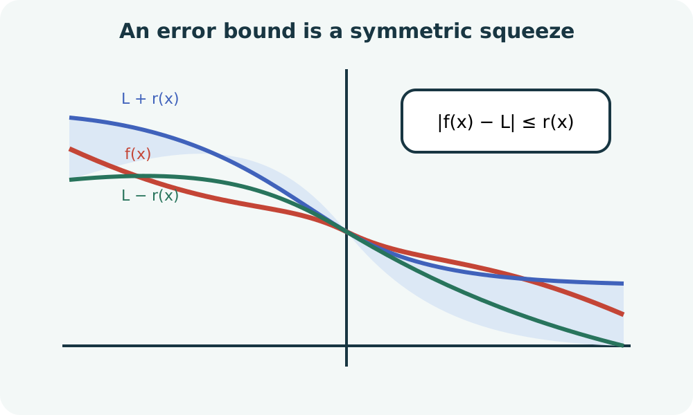
A highly useful form begins with $|f(x)-L|\le r(x)$ near $a$. Assume $r(x)\ge0$ and $\lim_{x\to a}r(x)=0$. The left side is the distance between the output and proposed limit. The inequality says this distance is no greater than a shrinking error allowance. Therefore $f(x)\to L$.

The absolute inequality is equivalent to $-r(x)\le f(x)-L\le r(x)$. Adding $L$ gives $L-r(x)\le f(x)\le L+r(x)$. Both outer functions approach $L$. The original Squeeze Theorem then applies. The absolute-value form is not a different theorem but a symmetric repackaging.

This form is often safer when multipliers can change sign. Instead of multiplying a three-part inequality by $x$, take absolute values and use product rules such as $|ab|=|a||b|$. Sign changes are absorbed into magnitudes. The goal becomes finding a simple nonnegative bound tending to zero. Many oscillatory limits follow this pattern.

Bounded oscillation times a shrinking factor

Consider $f(x)=x^2\sin\left(\frac{1}{x}\right)$ near zero. The sine factor oscillates infinitely often and has no limit as $x\to0$. Nevertheless, $-1\le\sin\left(\frac{1}{x}\right)\le1$. Since $x^2\ge0$, multiplication preserves inequality direction. Thus $-x^2\le f(x)\le x^2$.

Both bounds approach zero. The theorem gives $\lim_{x\to0}x^2\sin\left(\frac{1}{x}\right)=0$. The oscillation never settles, but its amplitude is compressed into an interval of width $2x^2$. That width approaches zero. The shrinking factor controls the bounded irregular factor.

The absolute-value method states the same argument compactly. Since $\left|\sin\left(\frac{1}{x}\right)\right|\le1$, we have $\left|x^2\sin\left(\frac{1}{x}\right)\right|\le x^2$. The right side approaches zero. This pattern generalizes to any bounded factor multiplied by a factor tending to zero. The bounded factor need not have its own limit.

A general bounded-times-zero result

Suppose $u(x)$ is bounded near $a$, meaning $|u(x)|\le M$ for some constant $M>0$. Suppose $v(x)\to0$. Then $|u(x)v(x)|\le M|v(x)|$. The right side approaches zero. Therefore $u(x)v(x)\to0$.

This result is sometimes called the bounded-times-zero theorem. It follows directly from squeezing. The function $u$ may oscillate, jump, or otherwise lack a limit. Only a local bound is required. The function $v$ supplies the shrinking scale.

For example, $x\cos\left(\frac{1}{x^2}\right)\to0$ as $x\to0$. The cosine magnitude is at most one, so the product magnitude is at most $|x|$. Another example is $x^3\arctan\left(\frac{1}{x}\right)$ because arctangent is bounded by $\frac{\pi}{2}$ in magnitude. Its absolute product is bounded by $\frac{\pi}{2}|x|^3$. Recognizing bounded factors is a reusable design skill.

Inequality operations require sign control

Adding the same expression to all parts of an inequality preserves order. Multiplying by a positive quantity preserves order. Multiplying by a negative quantity reverses every inequality. Taking reciprocals of positive quantities reverses order. Each transformation must state or establish the relevant sign.

Suppose $-1\le q(x)\le1$. Multiplying by $x$ is unsafe across a two-sided neighborhood of zero because $x$ changes sign. For $x>0$, it gives $-x\le xq(x)\le x$. For $x<0$, the directions reverse. Absolute values avoid splitting the proof because $|xq(x)|\le|x|$ holds on both sides.

Squaring inequalities also needs care. From $-2\le y\le1$, it does not follow that $4\le y^2\le1$. Squaring is not increasing across negative and positive values. Work with absolute magnitudes or known nonnegative intervals. Valid squeezing begins with valid order.

Designing useful bounds

Begin by identifying the troublesome factor. Trigonometric functions often have standard magnitude bounds such as $|\sin u|\le1$ and $|\cos u|\le1$. Rational expressions may be bounded by comparing denominator size. Radicals may be compared after establishing nonnegativity. Geometry can provide area or length inequalities.

Next isolate a factor that tends to zero or a pair of simpler functions with known limits. The bound should retain enough dependence on $x$ to collapse. A constant bound such as $|f(x)|\le10$ proves boundedness but not convergence to zero. Replacing a complicated term with something too coarse can destroy the needed shrinking information. Bound design balances simplicity and sharpness.

Finally verify locality and common limits. Write the interval on which denominators are nonzero and signs are known. Compute outer limits explicitly. If they differ, the squeeze does not determine the target limit. A failed bound may still suggest how to construct a tighter one.

Deriving the sine-over-angle limit

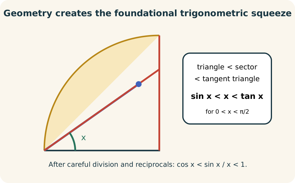
For $0<x<\frac{\pi}{2}$, unit-circle geometry gives $\sin x<x<\tan x$. The areas of an inscribed triangle, sector, and circumscribed triangle establish this order. Radian measure is essential because sector area is $\frac{x}{2}$ for a unit circle. The angle $x$ is dimensionless in the analytic formula. Degree measure would introduce a scale factor.

Divide the inequality by positive $\sin x$ to obtain $1<\frac{x}{\sin x}<\frac{1}{\cos x}$. Every quantity is positive on the interval. Taking reciprocals reverses order, giving $\cos x<\frac{\sin x}{x}<1$. As $x\to0^+$, both outer functions approach one. Therefore the right-hand limit is one.

The ratio $\frac{\sin x}{x}$ is even because replacing $x$ by $-x$ changes both numerator and denominator signs. Its left-hand behavior matches its right-hand behavior. Consequently $\lim_{x\to0}\frac{\sin x}{x}=1$. This foundational limit supports derivatives of sine and cosine. The Squeeze Theorem transfers geometric information into calculus.

A related trigonometric limit

Consider $\lim_{x\to0}\frac{1-\cos x}{x}$. Multiply numerator and denominator by $1+cos x$. The expression becomes $\frac{\sin^2x}{x(1+cos x)}$. Rewrite it as $\frac{\sin x}{x}\cdot\frac{\sin x}{1+cos x}$. Each factor now has a recognizable limit.

The first factor approaches one by the sine-over-angle result. The second approaches zero because its numerator approaches zero and denominator approaches two. Therefore the product approaches zero. This solution uses limit laws after a squeeze-established foundational limit. It illustrates how one theorem result becomes a tool in later algebra.

A direct bound is also possible. Since $1-cos x=2\sin^2\left(\frac{x}{2}\right)$ and $|\sin u|\le|u|$, the numerator is at most $\frac{x^2}{2}$ in magnitude. Dividing by $|x|$ gives a bound $\frac{|x|}{2}$. The right side approaches zero. Multiple valid approaches can illuminate different structures.

One-sided squeezing

The theorem has one-sided forms. For a right-hand limit, inequalities need only hold when $a<x<a+\delta_0$. Both outer right-hand limits must equal $L$. The conclusion is $\lim_{x\to a^+}f(x)=L$. A left-hand version is analogous.

One-sided bounds are useful when sign changes across the point. The unit-circle argument for sine begins on the positive side because lengths and areas are compared for positive angles. Symmetry then supplies the other side. Alternatively, separate left-hand inequalities could be developed. The proof structure remains local.

To establish a two-sided limit from one-sided squeezes, both one-sided limits must exist and agree. A right-hand squeeze alone cannot determine the left-hand behavior. The two sides may require different bounding functions. State the direction in every limit symbol. Directional precision prevents a half-proof from being mistaken for a full conclusion.

Squeezing at infinity

The theorem also applies as $x\to\infty$. Suppose $g(x)\le f(x)\le h(x)$ for all sufficiently large $x$. If both outer functions approach $L$, then $f(x)$ approaches $L$. The phrase sufficiently large replaces the punctured neighborhood around a finite point. The trapping logic is unchanged.

For example, consider $\frac{\sin x}{x}$ as $x\to\infty$. Since $|\sin x|\le1$, we have $\left|\frac{\sin x}{x}\right|\le\frac{1}{x}$ for positive large $x$. The right side approaches zero. Therefore the target approaches zero. Oscillation is compressed by the growing denominator.

Another example is $\frac{x+sin x}{x}=1+\frac{\sin x}{x}$. The bounded oscillatory correction approaches zero. The whole expression approaches one. This is an asymptotic statement: the linear term $x$ dominates the bounded perturbation. Squeezing formalizes that dominance.

Sequence version

Sequences have a corresponding theorem. If $a_n\le b_n\le c_n$ for all sufficiently large $n$ and both $a_n$ and $c_n$ approach $L$, then $b_n$ approaches $L$. The index $n$ takes integer values rather than varying continuously. “Sufficiently large” means beyond some index $N$. The proof uses the same tolerance logic.

Consider $b_n=\frac{\sin n}{n}$. Since $|\sin n|\le1$, we have $|b_n|\le\frac{1}{n}$. The sequence $\frac{1}{n}$ approaches zero. Therefore $b_n$ approaches zero. The numerator does not need to converge.

The sequence form becomes important in infinite series and numerical analysis. Error sequences are often trapped by simpler remainders. If an absolute error is at most a bound tending to zero, approximation convergence follows. The absolute-value squeeze is therefore a general error-control principle. It links introductory limits with later convergence arguments.

Quantitative bounds and error estimates

Squeezing can do more than prove a limit. If $|f(x)-L|\le r(x)$, then $r(x)$ is an explicit error bound. Choosing inputs that make $r(x)<\varepsilon$ guarantees desired accuracy. The same inequality provides both qualitative convergence and quantitative control. This is useful in approximation and computation.

For $f(x)=x^2\sin\left(\frac{1}{x}\right)$, the limit is zero and error magnitude is at most $x^2$. To guarantee $|f(x)|<0.001$, it is sufficient to require $x^2<0.001$. Thus $|x|<\sqrt{0.001}$ works. This distance is approximately $0.0316$. The actual function may satisfy the tolerance for additional inputs, but the bound provides a guaranteed region.

The estimate can be conservative. A broad outer bound ignores cancellations or finer structure. A tighter valid bound can produce a larger guaranteed input region. Quantitative squeezing therefore rewards careful inequality design. It turns theorem use into an optimization of proof information.

Common mistakes and repairs

One mistake finds two bounds but does not show that the target lies between them near the point. Write the inequality explicitly and state its neighborhood. Another mistake computes different outer limits and still declares a squeeze. Different limits provide only a range. A unique conclusion requires agreement.

A second mistake multiplies inequalities without checking sign. Use an interval where the multiplier sign is fixed or switch to absolute values. Another mistake assumes a bounded target must converge. Functions such as $\sin\left(\frac{1}{x}\right)$ are bounded near zero but do not have a limit. The bounding corridor must collapse.

A third mistake invokes the theorem when direct limit laws already solve the problem but gives no bounds. The theorem is not a phrase that replaces reasoning. It is a transfer of a known limit through verified inequalities. Name the lower function, upper function, common limit, and local ordering. A short solution can still be complete.

Practice and retrieval

Evaluate $\lim_{x\to0}x^3\cos\left(\frac{5}{x}\right)$. Construct an absolute-value bound. Explain why the cosine factor need not have a limit. State the target value before proving it. Give a sufficient input condition for making the magnitude below $10^{-6}$.

Evaluate $\lim_{x\to0}x^2\ln\left(1+\frac{1}{x^2}\right)$. Introduce $u=\frac{1}{x^2}$ or use a known logarithmic inequality to create a useful comparison. Explain why a constant bound is insufficient. Track signs and domains carefully. State whether the argument is two-sided.

Finally, prove $\lim_{x\to0}\frac{\tan x}{x}=1$ using the sine-over-angle limit and continuity of cosine. Identify every factor. Explain where denominator nonzero conditions are used. Then describe how the result depends on radian measure. This task combines a prior squeeze result with ordinary limit laws.

Solutions and reasoning

Because $|\cos(5/x)|\le1$, we have $|x^3\cos(5/x)|\le|x|^3$. The right side approaches zero, so the target limit is zero. Cosine oscillation does not need to settle because it is bounded. Requiring $|x|^3<10^{-6}$ gives the sufficient condition $|x|<0.01$. The bound is valid on both sides of zero.

For $u>0$, $\ln(1+u)\le u$ is too coarse here because it yields a constant after multiplication. A sharper asymptotic rewrite uses $x^2\ln(1+x^{-2})=\frac{\ln(1+u)}{u}$ with $u=x^{-2}\to\infty$. Since logarithm grows more slowly than a linear function, this ratio approaches zero, which can be established through integral or derivative bounds developed later. Within a strictly foundational squeeze lesson, an available bound such as $\ln(1+u)\le C\sqrt{u}$ for sufficiently large $u$ gives magnitude at most $C|x|$. The two-sided conclusion follows because the expression depends on $x^2$.

Write $\frac{\tan x}{x}=\frac{\sin x}{x}\cdot\frac{1}{\cos x}$. The first factor approaches one by the geometric squeeze. The second approaches one by continuity because cosine approaches one and stays nonzero near zero. The product limit is one. The sine-over-angle foundation assumes radian measure, so the result inherits that convention. Degrees would introduce a conversion factor.

Connection forward

The Squeeze Theorem supports foundational trigonometric limits used to derive trigonometric derivatives. It also provides error estimates for approximations and asymptotic comparisons. Later analysis uses closely related comparison principles for sequences, series, integrals, and differential equations. The underlying habit is to replace an inaccessible object with controlled neighbors. That habit extends far beyond calculus limits.

Formal epsilon-delta proofs also become easier to understand through squeezing. A bound on $|f(x)-L|$ converts a difficult output expression into a simpler one. Solving the simpler inequality for input distance produces a delta choice. The theorem packages this reasoning when outer limits are already known. It is therefore both a computational shortcut and a proof principle.

Carry forward a four-step routine. Identify irregular behavior, construct valid local bounds, compute outer limits, and verify that they agree. Use absolute values when signs complicate multiplication. State neighborhoods and one-sided directions explicitly. When the corridor truly collapses, the target limit follows with no room for ambiguity.