Estimating Limits from Graphs, Tables, and Formulas

A limit asks a deceptively simple question: what value is a function approaching as its input approaches a particular number?

That question matters because the behavior near a point can be meaningful even when the function behaves differently—or is not defined at all—at the point itself. This distinction is one of the ideas that led to the development of calculus.

Functions can be presented as formulas, tables, graphs, or verbal models. A reliable estimate of a limit should therefore not depend on one representation or one visual habit. Instead, we need to recognize the same underlying behavior in several forms and understand what each representation can—and cannot—tell us.

Learning objectives

By the end of this lesson, you should be able to:

• estimate a two-sided limit from a table;
• estimate a two-sided limit from a graph;
• use direct substitution as a first diagnostic for a formula;
• distinguish a limit from the value of the function at the point;
• recognize when left- and right-hand behavior disagree;
• choose informative numerical inputs when constructing a table; and
• explain why numerical and graphical evidence can support a limit estimate without necessarily proving it.

The object being estimated

The statement

$$\lim_{x\to a}f(x)=L$$

means that the values of $f(x)$ approach $L$ as $x$ approaches $a$.

The key word is approaches. To investigate the limit, we examine values of $x$ close to $a$ rather than relying on what happens exactly at $a$.

In particular,

$$x\to a$$

does not mean

$$x=a.$$

The limit concerns nearby behavior.

Approaching from the left and from the right

There are two ways for values of $x$ to move toward a number $a$ on the number line.

When $x$ approaches $a$ from the left, we use values that are less than $a$ and move progressively closer to it. We write

$$x\to a^-.$$

For example, if $a=2$, the sequence

$$1.9,\ 1.99,\ 1.999,\ldots$$

approaches $2$ from the left.

When $x$ approaches $a$ from the right, we use values that are greater than $a$ and move progressively closer to it. We write

$$x\to a^+.$$

For example,

$$2.1,\ 2.01,\ 2.001,\ldots$$

approaches $2$ from the right.

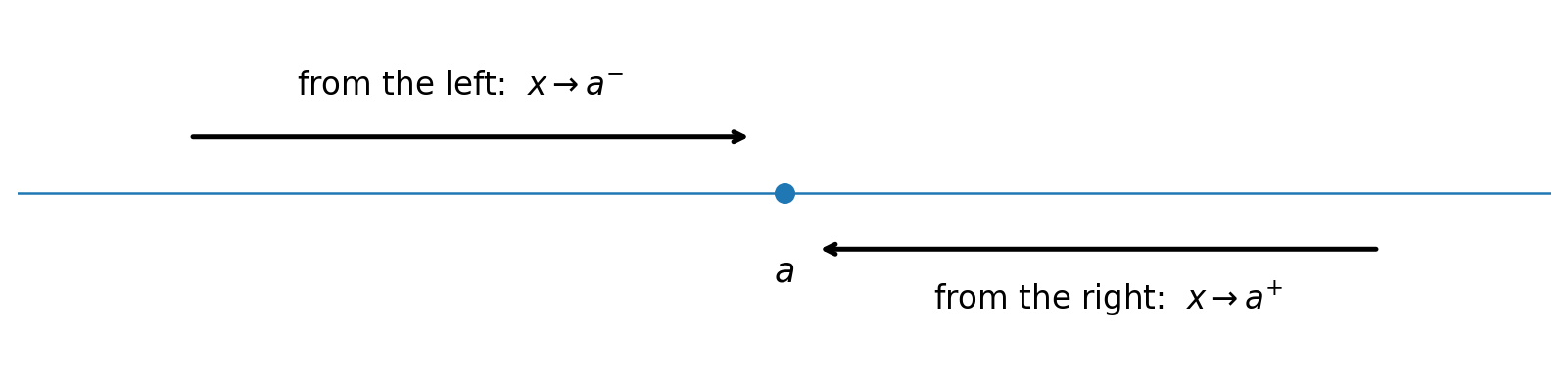
The superscript minus and plus signs describe the direction of approach. They do not mean that the input itself is negative or positive.

We use the same idea to describe what happens to the function values:

$$\lim_{x\to a^-}f(x)=L$$

is the left-hand limit, and

$$\lim_{x\to a^+}f(x)=L$$

is the right-hand limit.

A two-sided limit exists only when both sides approach the same value:

$$\lim_{x\to a^-}f(x) = \lim_{x\to a^+}f(x) = L.$$

This separates two questions that students often combine:

1. What happens to $f(x)$ as $x$ approaches $a$?
2. What is $f(a)$?

Those questions may have the same answer, but they do not have to.

Estimating from a table

A table lets us approach the target input numerically.

Suppose we want to estimate

$$\lim_{x\to2}f(x).$$

A useful table should contain values on both sides of $2$:

The table’s gridlines should remain thin and unobtrusive: strong enough to separate the numerical values, but not so heavy that they compete with the mathematics.

The goal is not merely to collect values close to $2$. We want to see whether the corresponding outputs settle toward the same number from both directions.

Inputs that are too coarse can conceal important behavior. On the other hand, inputs chosen extremely close to the target can sometimes expose calculator or floating-point rounding limitations. A good numerical investigation uses several progressively closer values and looks for a stable pattern.

When a table shows that a two-sided limit does not exist

A table can also reveal disagreement between the two sides.

Estimating from a graph

A graph gives a geometric version of the same process.

To estimate

$$\lim_{x\to a}f(x),$$

imagine tracing the graph toward $x=a$ from the left and asking which vertical coordinate the curve approaches. Then repeat the process from the right.

If both sides approach the same height $L$, the graph supports

$$\lim_{x\to a}f(x)=L.$$

The point value can be different

A graph may contain an open circle at the limiting location and a filled point somewhere else at the same $x$-coordinate.

For example, imagine that as $x$ approaches $2$, the curve approaches the open point $(2,4)$, but the graph contains a filled point at $(2,7)$.

Then

$$\lim_{x\to2}f(x)=4$$

while

$$f(2)=7.$$

There is no contradiction. The first statement describes nearby behavior; the second describes the value assigned at the point.

Graphs provide evidence, not infinite resolution

A graph is only a representation drawn at a particular scale.

A viewing window can hide:

• a narrow spike;
• rapid oscillation;
• a nearby discontinuity;
• behavior occurring below the graph’s visible resolution.

For that reason, graphical evidence can provide a convincing estimate without constituting an exact evaluation by itself.

Tables and graphs are valuable because they reveal numerical and geometric behavior, but they sample only finitely many values or display the function at finite visual resolution. When a formula is known and an analytic method is available, the limit should be evaluated by calculation. The table and graph then serve as supporting representations of the result rather than substitutes for the calculation.

This limitation is important. Calculus ultimately needs definitions and analytical techniques precisely because pictures and finite tables cannot reveal behavior at every possible scale.

Estimating from a formula

When a function is given algebraically, direct substitution is the first diagnostic.

Suppose we want

$$\lim_{x\to a}f(x).$$

First evaluate the expression at $x=a$.

Case 1: substitution gives an ordinary real number

For example,

$$\lim_{x\to2}(x^2+3x-1).$$

Substituting $x=2$ gives

$$2^2+3(2)-1=9.$$

Because polynomials are continuous,

$$\boxed{\lim_{x\to2}(x^2+3x-1)=9}.$$

In this case, the function value and the limit agree.

Case 2: substitution gives an indeterminate form

Consider the previous example:

$$f(x)=\frac{x^2-4}{x-2}.$$

If we try to evaluate

$$\lim_{x\to2}\frac{x^2-4}{x-2}$$

by direct substitution, we obtain

$$\frac{2^2-4}{2-2} = \frac00.$$

This is not the value of the limit.

An indeterminate form such as $\frac{0}{0}$ tells us to look more closely at the algebra. In some cases, a common factor is responsible for the undefined expression and can be removed before the limit is evaluated. The next section develops exactly that situation.

Removable discontinuities

Return to

$$f(x)=\frac{x^2-4}{x-2}.$$

We already know that direct substitution at $x=2$ produces the indeterminate form $\frac{0}{0}$. Factor the numerator:

$$x^2-4=(x-2)(x+2).$$

For every $x\neq2$,

$$\frac{x^2-4}{x-2} = \frac{(x-2)(x+2)}{x-2} = x+2.$$

The factor responsible for the undefined expression cancels. The original function remains undefined at $x=2$, but everywhere sufficiently near $2$ it follows the same line as $y=x+2$.

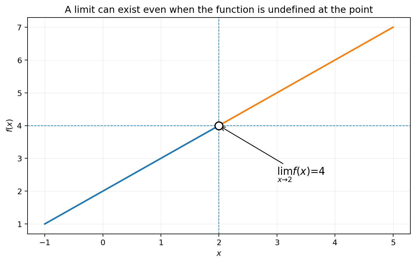
As shown in the removable-discontinuity graph below, the curve approaches $(2,4)$ from both sides even though the function itself is undefined at $x=2$.

We can therefore calculate

$$\begin{aligned} \lim_{x\to2}\frac{x^2-4}{x-2} &= \lim_{x\to2}(x+2)\\ &=4. \end{aligned}$$

Thus,

$$\boxed{\lim_{x\to2}\frac{x^2-4}{x-2}=4}.$$

This is a removable discontinuity. The discontinuity can be removed by defining $f(2)=4$, which would make the resulting function continuous at $x=2$.

Factoring is therefore especially useful when direct substitution produces an indeterminate form and the numerator and denominator contain a common factor.

Nonremovable discontinuities

Not every undefined expression can be repaired by cancellation.

Consider

$$f(x)=\frac{x-2}{x^2-4}.$$

Direct substitution at either $x=2$ or $x=-2$ encounters a zero in the denominator. Factor the denominator:

$$x^2-4=(x-2)(x+2).$$

For $x\neq2$,

$$f(x) = \frac{x-2}{(x-2)(x+2)} = \frac{1}{x+2}.$$

At $x=2$, the common factor cancels, so the discontinuity there is removable:

$$\lim_{x\to2}f(x) = \lim_{x\to2}\frac{1}{x+2} = \frac14.$$

At $x=-2$, however, no factor in the numerator can cancel the factor $x+2$ in the denominator. The simplified expression

$$\frac{1}{x+2}$$

still has a zero denominator at $x=-2$.

As the graph below shows, the function decreases without bound on one side of $x=-2$ and increases without bound on the other. The vertical line $x=-2$ is a vertical asymptote.

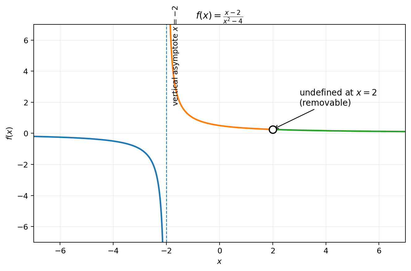
Specifically,

$$\lim_{x\to-2^-}f(x)=-\infty$$

while

$$\lim_{x\to-2^+}f(x)=+\infty.$$

Because the two sides do not approach the same value,

$$\boxed{\lim_{x\to-2}\frac{x-2}{x^2-4}\text{ does not exist}.}$$

The denominator has a higher polynomial degree than the numerator, which is a useful warning that not every denominator factor can be canceled. More precisely, factorization shows which discontinuities are removable: a zero-producing denominator factor is removable only when the same factor also occurs in the numerator and cancels. Here, $(x-2)$ cancels but $(x+2)$ does not, so $x=2$ is removable while $x=-2$ is nonremovable.

The graph makes this distinction visible: at $x=2$ there is a single undefined point on an otherwise finite curve, whereas near $x=-2$ the function grows without bound.

Connecting the representations

Tables, graphs, and formulas are not three unrelated ways to perform a limit problem. They are different views of the same underlying question:

What is the function doing as the input gets arbitrarily close to the target?

For the limit

$$\lim_{x\to2}f(x) = \lim_{x\to2}\frac{x^2-4}{x-2},$$

the three representations tell a consistent story:

• Table: outputs approach $4$ from both sides.
• Graph: the curve approaches the point $(2,4)$ even though the original function is undefined there.
• Formula: factoring shows that for every nearby $x\neq2$, the expression equals $x+2$.

Agreement among representations strengthens our understanding because each representation reveals something different.

The table makes the approach visible numerically.
The graph above makes it visible geometrically.
The algebra explains why the pattern occurs and, when the formula is known, provides the analytic evaluation of the limit.

Tables and graphs are therefore important evidence and excellent tools for building intuition, checking work, and estimating behavior. The calculation is what establishes the exact value of the limit when the function is known and can be analyzed algebraically.

Choosing the right evidence

When estimating a limit, ask:

1. What value of $x$ am I approaching?
2. Have I examined behavior from the left?
3. Have I examined behavior from the right?
4. Do both sides appear to approach the same output?
5. Am I accidentally using $f(a)$ as though it were automatically the limit?
6. Is the representation precise enough to support the conclusion?
7. If a formula gives an indeterminate form, what additional analysis is available?

A strong limit argument is not merely a guess at a graph or a sequence of calculator entries. It explains why the available evidence supports the proposed limiting behavior.

Test Your Knowledge

1. Limit versus function value

A table shows that $f(x)\to5$ from both sides as $x\to1$, while

$$f(1)=-2.$$

Determine

$$\lim_{x\to1}f(x)$$

and $f(1)$.

Solution

The nearby values approach $5$ from both sides, so

$$\lim_{x\to1}f(x)=5.$$

The assigned point value is

$$f(1)=-2.$$

These values differ because the limit describes nearby behavior while $f(1)$ describes the value at the point.

2. Reading two sides

As $x$ approaches $4$ from the left, a graph approaches $y=3$. As $x$ approaches $4$ from the right, it approaches $y=3$. A filled point appears at $(4,8)$.

What are

$$\lim_{x\to4}f(x)$$

and $f(4)$?

Solution

Both sides approach $3$, so

$$\lim_{x\to4}f(x)=3.$$

The filled point gives the function value:

$$f(4)=8.$$

3. When the sides disagree

Suppose

$$\lim_{x\to2^-}f(x)=-1$$

and

$$\lim_{x\to2^+}f(x)=6.$$

Does the two-sided limit exist?

Solution

No. A two-sided limit exists only when the left- and right-hand limits agree. Since

$$-1\neq6,$$

the limit

$$\lim_{x\to2}f(x)$$

does not exist.

4. Direct substitution

Estimate

$$\lim_{x\to3}(2x^2-x+4).$$

Solution

Direct substitution gives

$$2(3)^2-3+4=18-3+4=19.$$

Because the expression is a polynomial,

$$\lim_{x\to3}(2x^2-x+4)=19.$$

5. Interpreting an indeterminate form

Direct substitution into a limit produces $\frac{0}{0}$. Which conclusion is justified?

A. The limit is $0$.
B. The limit does not exist.
C. The limit is infinite.
D. Direct substitution has not determined the limit.

Solution

D. The form $\frac{0}{0}$ is indeterminate. Additional analysis is required.

6. Evaluating numerical evidence

You are estimating $\lim_{x\to5}f(x)$. A table contains only the inputs

$$4,\ 4.5,\ 4.9,\ 4.99.$$

What important information is missing?

Solution

Every listed input approaches $5$ from the left. To estimate a two-sided limit, we also need values greater than $5$ that approach from the right, such as $5.01$, $5.1$, and $5.5$.