Continuity at a Point

Continuity aligns a function’s nearby behavior with its assigned value. The phrase “draw the graph without lifting a pencil” offers useful intuition but does not supply a reliable test. Limits make the idea precise at individual points and across intervals. The definition also identifies why continuity fails and whether one changed value can repair it. This lesson turns that definition into a repeatable evidence-based process.

Interpret continuity as agreement

A limit describes what function values approach near an input. A function value describes what the rule assigns exactly at that input. These two quantities can exist independently and can disagree. Continuity requires them to align. That distinction is why evaluating a point is not the same as evaluating a limit.

Suppose $f(x)=x^2$ for every $x\ne2$ but $f(2)=100$. Nearby values still approach four because changing one isolated value does not change punctured-neighborhood behavior. Thus $\lim_{x\to2}f(x)=4$ while $f(2)=100$. The function is not continuous at two. Its limit exists even though continuity fails.

Continuity is a local stability condition. Small input changes near $a$ produce output values close to $f(a)$. This does not mean the entire graph is flat or slowly varying. It means no fixed jump separates the nearby behavior from the assigned value at that point. The amount of input control required may differ from one point to another.

Apply the three-part test in order

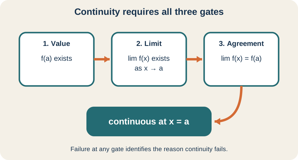
A function $f$ is continuous at $x=a$ when three conditions hold. First, $f(a)$ must be defined. Second, the two-sided limit $\lim_{x\to a}f(x)$ must exist. Third, that limit must equal $f(a)$. Failure of any one condition means discontinuity at the point.

The compact equation $\lim_{x\to a}f(x)=f(a)$ contains all three conditions implicitly. Its left side must exist for the equality to be meaningful. Its right side must also exist. The equality then supplies agreement. In written justification, expanding the compact statement into three checks makes the evidence visible.

Use the test in its stated order. Record the function value without assuming that it predicts nearby behavior. Compute one-sided limits when a formula, graph, table, or domain changes at the point. Name the common two-sided limit only when the one-sided limits agree. Compare the two independently obtained quantities last.

Use one-sided limits at interior points

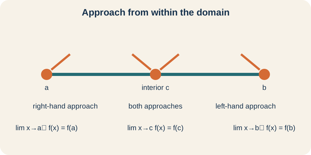
At an interior domain point, a two-sided limit exists only when both one-sided limits exist and agree. The left-hand limit is written $\lim_{x\to a^-}f(x)$, where the superscript minus indicates inputs less than $a$. The right-hand limit is $\lim_{x\to a^+}f(x)$, where the superscript plus indicates inputs greater than $a$. These signs describe approach direction rather than positive or negative function values. Their equality is evidence for one common nearby behavior.

Piecewise functions make this test especially important. Use the left formula for the left-hand limit and the right formula for the right-hand limit. Use whichever piece includes equality to determine the actual function value. Do not substitute the boundary into both formulas and call the results function values. One formula may govern nearby inputs without governing the boundary itself.

Consider $g(x)=mx+2$ for $x<1$ and $g(x)=x^2+3$ for $x\ge1$. The left-hand limit is $m+2$, while the right-hand limit and value are both four. Continuity requires $m+2=4$. Therefore $m=2$. This parameter makes both approaches and the assigned value agree.

Treat endpoints relative to the domain

Continuity is always relative to a function’s domain. At the left endpoint $a$ of a closed domain interval, no allowed inputs approach from the left. Continuity therefore requires $\lim_{x\to a^+}f(x)=f(a)$. At the right endpoint $b$, the condition is $\lim_{x\to b^-}f(x)=f(b)$. Interior points still require a two-sided limit.

The real square-root function illustrates the convention. Its domain is $[0,\infty)$, so zero is a left endpoint. The right-hand limit $\lim_{x\to0^+}\sqrt{x}=0$ equals the value $\sqrt{0}=0$. Therefore square root is continuous at zero on its real domain. A nonexistent left-domain approach is not a failed condition.

These endpoint conventions matter for interval theorems. Continuity on $[a,b]$ means two-sided continuity at every interior point, right continuity at $a$, and left continuity at $b$. The Extreme Value Theorem and Intermediate Value Theorem use this definition. Endpoint conditions are not exceptions invented for convenience. They express approach using only inputs where the function is defined.

Classify removable and jump discontinuities

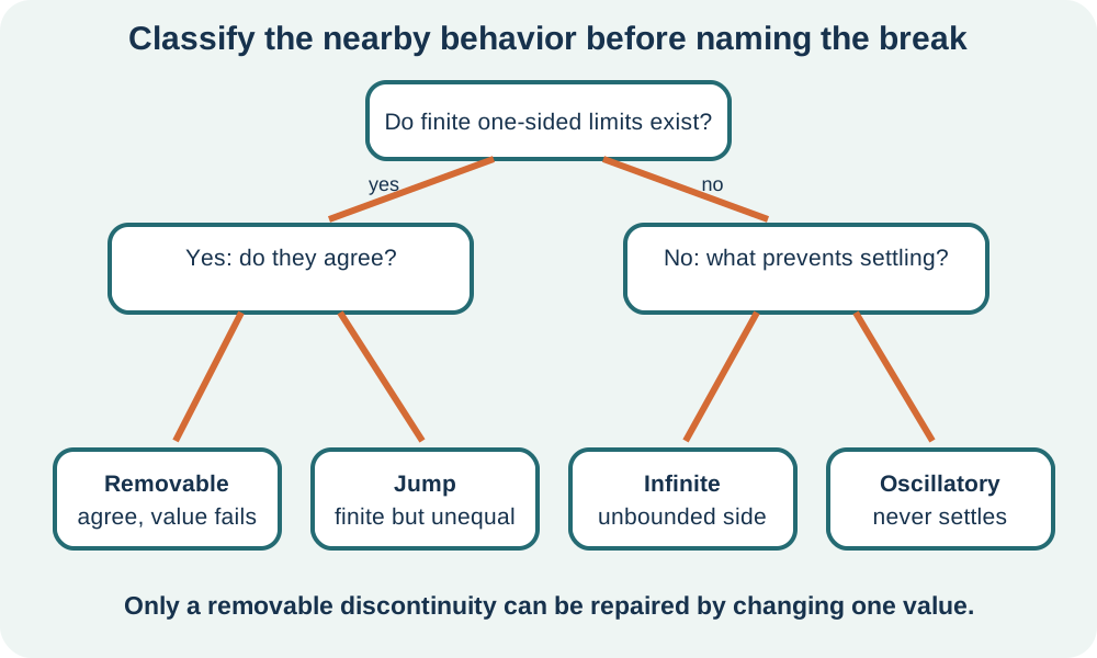
A removable discontinuity occurs when the two-sided limit exists but the function value is missing or unequal. The nearby behavior has one target, so changing one point can create agreement. The graph often appears as a hole, possibly accompanied by a filled point elsewhere at the same input. The adjective removable describes a possible redefinition, not automatic cancellation. The original function remains discontinuous until the value is repaired.

For $f(x)=\frac{x^2-9}{x-3}$ with $x\ne3$, factor the numerator as $(x-3)(x+3)$. Canceling the common factor for nearby nonzero denominators gives $x+3$. Thus $\lim_{x\to3}f(x)=6$. Defining $f(3)=6$ repairs the discontinuity. Cancellation does not prove the original quotient was defined at three.

A jump discontinuity occurs when finite one-sided limits exist but differ. Changing the single function value cannot reconcile two different nearby targets. For example, if the left-hand limit is four and the right-hand limit is six, no choice of $f(a)$ makes the two-sided limit exist. The failure occurs in neighborhood behavior rather than only at the point. Jump models can still be useful, but continuous theorems cannot cross the jump without additional analysis.

Classify infinite and oscillatory failures

An infinite discontinuity occurs when function values become unbounded from at least one side. Rational functions can produce this behavior near a noncanceled denominator zero. The notation $f(x)\to\infty$ describes unbounded growth, not approach to a real number named infinity. A vertical asymptote often accompanies the behavior. One-sided signs must still be checked because opposite sides can diverge differently.

An oscillatory discontinuity occurs when values continue varying without settling on one target. The function $\sin\left(\frac{1}{x}\right)$ near zero is the standard example. As $x$ approaches zero, the reciprocal input grows without bound and sine cycles indefinitely between negative one and one. The values remain bounded but have no limit. No single definition at zero can change that neighborhood behavior.

Distinguishing these types guides the response. A removable failure invites a repaired value. A jump may require a new piecewise transition model. Infinite behavior signals unbounded output or a domain boundary, while oscillation signals persistent variation at every scale. Classification should follow limit evidence rather than visual vocabulary alone.

Build continuity from known functions

Polynomials are continuous for every real input. Rational functions are continuous wherever their denominators are nonzero. Exponential and trigonometric functions are continuous throughout their natural real domains. Logarithmic and radical functions are continuous where their inputs satisfy their domain restrictions. These facts justify direct substitution only after the relevant domain condition has been checked.

Sums, differences, products, and constant multiples of continuous functions remain continuous where all components are defined. Quotients remain continuous where the denominator is nonzero. Compositions require continuity at two linked locations. If $g$ is continuous at $a$ and $f$ is continuous at $g(a)$, then $f\circ g$ is continuous at $a$. The outer function’s hypothesis must be checked at the inner output.

Consider $F(x)=\sqrt{5-x^2}$ at $x=1$. The inner polynomial is continuous and has value four. Square root is continuous at the positive input four. Therefore $\lim_{x\to1}\sqrt{5-x^2}=\sqrt{5-1^2}=2=F(1)$. This is justified substitution based on component continuity, not substitution used as an unsupported guess.

Relate continuity and differentiability

Differentiability at a point implies continuity there. A derivative supplies a finite local linear model, which forces function values to approach the assigned value. This implication is one-directional. Continuity alone does not guarantee that nearby change has one consistent slope. The hierarchy prevents the two concepts from being treated as synonyms.

The absolute-value function is continuous at zero. Both one-sided function limits equal zero, which matches $|0|=0$. Its left-hand slope is negative one and its right-hand slope is positive one. Because those derivative limits disagree, the derivative does not exist at zero. The corner is continuous but not differentiable.

Other continuous nondifferentiable behaviors include cusps, vertical tangents, and certain oscillations. Each preserves output agreement while failing a derivative requirement. When asked whether differentiability holds, continuity is a necessary preliminary check but not a complete proof. When differentiability is established, continuity follows automatically. State the direction of implication explicitly to avoid reversing it.

Express continuity as input-output control

The epsilon-delta definition makes stability quantitative. Continuity at $a$ means that for every output tolerance $\varepsilon>0$, there is an input tolerance $\delta>0$ such that $|x-a|<\delta$ guarantees $|f(x)-f(a)|<\varepsilon$. The Greek letter epsilon measures allowed output error. Delta measures how tightly the input must be controlled. Both quantities are positive.

For $f(x)=|x|$, the reverse triangle inequality gives $\big||x|-|a|\big|\le|x-a|$. Given an output tolerance $\varepsilon$, choose $\delta=\varepsilon$. Then $|x-a|<\delta$ immediately implies $\big||x|-|a|\big|<\varepsilon$. This proves continuity at every real $a$. The inequality translates the visual stability of absolute value into exact control.

The required delta can depend on the point and on epsilon. Continuity does not claim that one universal input tolerance works everywhere. It also does not claim small slopes or constant behavior. It claims that arbitrary output accuracy can be achieved through sufficiently tight local input control. This viewpoint becomes important in error propagation and numerical approximation.

Prove continuity with a reusable template

Start by stating that the point lies in the function’s domain. Identify known continuous component functions and the operations combining them. Verify denominator, logarithm, radical, and composition restrictions. Use justified limit laws to evaluate the nearby limit. Compare the limit explicitly with the function value.

For a rational function $R(x)=\frac{p(x)}{q(x)}$, suppose $q(a)\ne0$. Polynomials $p$ and $q$ are continuous, and the quotient theorem applies because the denominator limit is nonzero. Therefore $\lim_{x\to a}R(x)=\frac{p(a)}{q(a)}=R(a)$. The nonzero condition is a hypothesis rather than a footnote. If it fails, factorization or one-sided analysis may be needed.

For a piecewise function, modify the template at the joining input. Establish continuity of each formula on its own side. Compute left and right limits separately and compare them. Determine the function value from the equality-bearing piece. Conclude continuity only if all three quantities agree.

Diagnose common reasoning errors

Checking only that $f(a)$ exists proves just the first condition. Checking only that the limit exists proves nearby agreement but not agreement with the value. Direct substitution can be circular when continuity is the very fact under investigation. A smooth-looking sketch can conceal a hole or misplotted point. Name the evidence for every condition instead of relying on appearance.

Not every denominator zero produces a vertical asymptote. A common factor can produce a removable hole, while an uncanceled factor may produce unbounded behavior. Factor the expression for nearby inputs before classifying it. Preserve the original domain even after cancellation. Algebraic simplification changes the convenient formula, not the value that was originally undefined.

Do not assume that redefining one point can repair every break. A new point value cannot alter left-side or right-side neighborhood behavior. It repairs continuity only when those sides already approach one common finite limit. It cannot remove a jump, infinite divergence, or oscillation. This single-value test is a powerful classification check.

Practice the decision process

Classify $\frac{x^2-4}{x-2}$ at $x=2$. The original function value is undefined. For nearby $x\ne2$, factoring and canceling gives $x+2$, so the limit is four. The discontinuity is removable. Defining the missing value as four creates continuity.

Now consider a greatest-integer function at an integer such as three. Values approaching from the left have greatest integer two, while values approaching from the right have greatest integer three. The one-sided limits differ, so the two-sided limit does not exist. The assigned value at three cannot fix this disagreement. The discontinuity is a jump.

For independent work, build a piecewise linear function whose parameter must be chosen for continuity. Write the left-hand limit, right-hand limit, and function value on separate lines. Solve the equality condition and verify it by substitution. Then create a second piecewise example that no parameter value can repair because its side limits differ structurally. Explaining why repair is possible or impossible is more important than merely naming the type.

Connect continuity to interval theorems

The Intermediate Value Theorem turns continuity on a closed interval into an existence guarantee. If a target output lies between the endpoint outputs, a continuous function must attain it somewhere inside. A jump could skip the target, which explains why interval continuity is required. The theorem guarantees existence but not uniqueness. It also does not locate the input without further numerical work.

The Extreme Value Theorem uses the same closed-interval continuity hypothesis. It guarantees that absolute maximum and minimum values are attained. A bounded-looking open interval may fail to include its extremal boundary values. A discontinuity can likewise destroy attainment. The hypotheses explain the theorem’s force and its limitations.

Derivative theory will impose a stronger local requirement. Because differentiability implies continuity, a discontinuity automatically prevents differentiability at that point. A continuous point may still require slope analysis. Carry the three-condition continuity test forward before applying derivative theorems. This order builds calculus conclusions on verified foundations.

Sources and further study

OpenStax Calculus, Volume 1 develops limits, continuity, and discontinuity classifications. Its examples provide additional algebraic and graphical representations. Compare each example with the three-condition test used here. Identify the exact failed condition before reading its classification. Retrieval and prediction make the reference an active learning tool.

The AP Calculus AB course overview supplies curriculum alignment for limit and continuity reasoning. It emphasizes translating among graphical, numerical, analytical, and verbal representations. Practice expressing the same continuity conclusion in all four forms. Check theorem hypotheses whenever continuity supports a later claim. Representation fluency reduces dependence on memorized visual patterns.

Further study should connect continuity to root-finding and numerical error. Bisection uses continuity to preserve a sign-change bracket containing a root. Approximation methods depend on stable input-output behavior. Explore how a removable hole, jump, and vertical asymptote affect numerical sampling differently. These comparisons show why classification matters in computation as well as in graph analysis.