Intermediate Value Theorem

Continuity prevents a function from skipping an intermediate output while moving between two endpoint outputs. The Intermediate Value Theorem turns that intuition into a precise existence guarantee. It can prove that an equation has a solution even when no algebraic formula reveals the solution. It can also support a reliable numerical search. This lesson develops the theorem as an argument with hypotheses, conclusion, and limitations.

State the theorem with all hypotheses

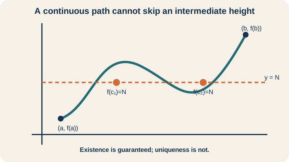
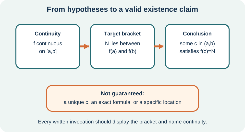
Suppose $f$ is continuous on the closed interval $[a,b]$. Let $N$ be a number between the endpoint outputs $f(a)$ and $f(b)$. The Intermediate Value Theorem guarantees at least one $c$ in the open interval $(a,b)$ such that $f(c)=N$. The letter $N$ names the target output. The letter $c$ names an input whose existence is guaranteed.

The phrase “between” allows either endpoint ordering. If $f(a)<f(b)$, require $f(a)<N<f(b)$ for a strictly intermediate target. If $f(b)<f(a)$, reverse the inequalities. A compact form is $\min\{f(a),f(b)\}<N<\max\{f(a),f(b)\}$. Endpoint equality can be handled trivially because an endpoint already supplies the target.

Every part of the statement carries information. Continuity must hold at every point of the closed interval, including one-sided endpoint continuity. The target must lie between the endpoint outputs. The conclusion gives at least one interior input, not necessarily exactly one. It does not provide a formula for that input.

Understand the geometric mechanism

Imagine tracing the graph continuously from $(a,f(a))$ to $(b,f(b))$. If the starting height lies below $N$ and the ending height lies above $N$, the path must cross the horizontal line $y=N$. A jump could pass from below to above without touching the line. Continuity excludes that escape. The crossing input is the theorem’s $c$.

The graph may cross the target many times. It may touch the target, reverse, and meet it again. The theorem does not require monotonicity. It only guarantees that the target is attained at least once. Uniqueness needs extra evidence, such as strict increase or a derivative with one sign.

The theorem is about output coverage. A continuous image of an interval contains every value between its endpoint outputs. This statement does not mean the graph stays numerically between those two outputs throughout the interval. It may rise above both or fall below both and still remain continuous. The theorem guarantees intermediate attainment, not a bound on all values.

Convert root questions into target questions

A root of $f$ is an input $c$ satisfying $f(c)=0$. Use the theorem with target $N=0$. If $f$ is continuous on $[a,b]$ and $f(a)$ and $f(b)$ have opposite signs, then zero lies between them. Therefore at least one root lies in $(a,b)$. The product condition $f(a)f(b)<0$ records the sign change compactly.

Consider $f(x)=x^3+x-1$ on $[0,1]$. A polynomial is continuous everywhere, so it is continuous on this closed interval. The endpoint values are $f(0)=-1$ and $f(1)=1$. Zero lies between negative one and positive one. Therefore some $c\in(0,1)$ satisfies $c^3+c-1=0$.

This argument proves existence without solving the cubic. It does not identify the exact root or even a decimal approximation. It also does not prove uniqueness by itself. In this example, $f'(x)=3x^2+1>0$, so the function is strictly increasing. That extra derivative evidence establishes that the guaranteed root is unique.

Write a complete theorem justification

A complete invocation has three parts. First, name why the function is continuous on the stated closed interval. Second, calculate endpoint outputs and show that the target lies between them. Third, state the theorem’s interior existence conclusion with the correct equation. Omitting any part weakens the logical chain.

For $g(x)=x^5-2x-3$ on $[1,2]$, polynomials establish continuity. The endpoint values are $g(1)=-4$ and $g(2)=25$. Because $-4<0<25$, zero is between the outputs. By the Intermediate Value Theorem, some $c\in(1,2)$ satisfies $g(c)=0$. This is a valid existence proof even if no simple exact form is found.

Avoid saying that “the function changes signs, so it has a root” without continuity. A discontinuous step can change from negative to positive while skipping zero. Also avoid claiming that the root equals the midpoint. Endpoint evidence brackets a solution but does not locate it exactly. The theorem’s vocabulary should match the strength of its conclusion.

Recognize why continuity is indispensable

Define $h(x)=-1$ for $x<0$ and $h(x)=1$ for $x\ge0$. On $[-1,1]$, the endpoint outputs have opposite signs. Yet the function never equals zero. The jump at zero violates continuity on the interval. This counterexample shows that a sign change alone is insufficient.

A removable hole can also destroy a specific target conclusion. Suppose a continuous formula would equal $N$ at exactly one input, but that value is deleted and reassigned elsewhere. Endpoint outputs may still bracket $N$. The modified function can skip the target if no other crossing occurs. Continuity at every interval point prevents this single-point escape.

An infinite discontinuity creates another failure mode. The function $f(x)=\frac{1}{x}$ has endpoint values of opposite signs on $[-1,1]$ but is undefined at zero. It never takes the value zero. The domain break invalidates closed-interval continuity. Checking the domain is therefore part of checking the theorem.

Distinguish existence from uniqueness and location

Existence means at least one qualifying input is present. Uniqueness means exactly one is present. Location means identifying or approximating where it lies. The Intermediate Value Theorem supplies only the first conclusion. A rigorous solution should not silently upgrade it to the other two.

Strict monotonicity can add uniqueness. If $f'(x)>0$ throughout $(a,b)$, then $f$ is strictly increasing and cannot take the same target value twice. If $f'(x)<0$, it is strictly decreasing and the same conclusion follows. Derivative evidence supplements rather than replaces the continuity argument. The two theorems answer different logical questions.

Numerical algorithms add location. Bisection narrows a sign-change interval, while Newton’s method uses tangent-line approximations. Their convergence assumptions and error behavior differ. A theorem proving that a root exists is not itself an algorithm. Separating these roles makes both the proof and the computation clearer.

Turn the guarantee into bisection

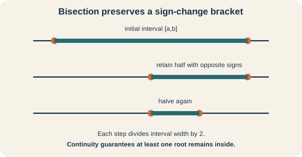
Bisection begins with a continuous function whose endpoint values have opposite signs. Compute the midpoint $m=\frac{a+b}{2}$. If $f(m)=0$, the root has been found. Otherwise retain the half-interval whose endpoint values still have opposite signs. Continuity guarantees that the retained bracket still contains at least one root.

Repeat the process on the smaller interval. Every iteration divides interval width by two. After $n$ halvings, the width is $\frac{b-a}{2^n}$. The midpoint’s distance from any root in the final bracket is at most half that width. This supplies an explicit error bound rather than only a plausible decimal.

For $f(x)=x^3+x-1$ on $[0,1]$, the midpoint is $0.5$. Its value is $-0.375$, so the sign change remains between $0.5$ and $1$. The next midpoint is $0.75$, where the function is positive. The bracket then becomes $[0.5,0.75]$, and continued halving narrows the root systematically. Each retained pair must be checked for opposite signs before the next step.

Plan precision before iterating

Suppose an initial bracket has width $b-a$. To guarantee a final width no greater than tolerance $T$, require $\frac{b-a}{2^n}\le T$. Solving for $n$ gives $n\ge\frac{\ln\left(\frac{b-a}{T}\right)}{\ln2}$. Round upward because the number of iterations must be a whole number. This planning prevents stopping by guesswork.

If the initial width is one and the desired width is at most $0.001$, then $2^n\ge1000$. Since $2^9=512$ and $2^{10}=1024$, ten halvings suffice. The final midpoint error is at most $0.0005$. State whether a reported tolerance refers to full bracket width or midpoint error. Mixing those quantities can overstate precision by a factor of two.

Bisection is reliable but not always fast. It uses only function signs and continuity, so it does not need derivatives. Newton’s method can converge more quickly near a suitable root but can fail from poor initial choices or small derivatives. A practical workflow may use bisection for safety and a faster method after a secure bracket is known. Reliability and speed are separate algorithmic qualities.

Apply the theorem to nonzero targets

The target need not be zero. Suppose temperature $T(t)$ varies continuously from $18\,^{\circ}\mathrm{C}$ at $t=0\,\mathrm{h}$ to $26\,^{\circ}\mathrm{C}$ at $t=3\,\mathrm{h}$. Because $22\,^{\circ}\mathrm{C}$ lies between those endpoint temperatures, the theorem guarantees a time $c\in(0,3)$ hours with $T(c)=22\,^{\circ}\mathrm{C}$. The conclusion assumes a continuous temperature model. It does not say when the event occurs.

Calibration provides another application. If a continuous sensor response is $1.2\,\mathrm{V}$ at one reference input and $4.8\,\mathrm{V}$ at another, every voltage between those readings occurs at some intermediate input. This supports existence of an input producing $3.0\,\mathrm{V}$. It does not guarantee one-to-one calibration. Monotonicity is needed to ensure one unique input per output.

Equilibrium problems can be written the same way. If a continuous net-force function is negative at one position and positive at another, some intermediate position has zero net force. That position is an equilibrium candidate. Stability requires additional information about nearby force direction or potential curvature. The theorem supplies existence, not dynamical classification.

Use tables and graphs without weakening rigor

A table can provide endpoint evidence if the displayed values are reliable. Choose two inputs whose function outputs bracket the target. Then separately justify continuity on the entire interval between those inputs. A table alone cannot establish continuity at unlisted points. It also cannot prove uniqueness unless additional structure is known.

A graph can suggest a bracket and reveal likely multiple crossings. However, pixel resolution can hide holes, jumps, or narrow oscillations. Use the graph to form a conjecture rather than as the sole continuity proof. Identify the analytic function family or stated model assumption that provides continuity. Then write the endpoint comparison numerically or symbolically.

Multiple representations can strengthen an argument. A formula establishes continuity, a table supplies a narrow bracket, and a graph communicates the crossing. Each representation answers a different question. Agreement among them supports confidence without changing the theorem’s hypotheses. State which evidence performs which logical role.

Diagnose common theorem errors

The first error is forgetting to establish continuity on the entire closed interval. Continuity only at endpoints is insufficient. The second error is computing endpoint values without showing the target lies between them. The third is reporting an endpoint as the guaranteed interior $c$ when the theorem’s strict target form assumes an interior solution. A complete proof avoids all three gaps.

Another error is claiming exactly one solution. A continuous oscillating function may cross the target many times. The theorem’s words “at least one” should appear in the conclusion. If uniqueness matters, add monotonicity or another injectivity argument. Never treat a sketch showing one visible crossing as proof that others do not exist.

A final error is confusing a bracket with an approximation of known accuracy. Saying a root lies in $[1,2]$ is an interval guarantee, not a decimal estimate. Reporting the midpoint $1.5$ should include an error no greater than $0.5$ for that bracket. Further bisection improves the bound. Precision belongs to the width of verified evidence.

Practice a complete existence argument

Show that $x^3-4x+1=0$ has a solution on $[0,1]$. The polynomial is continuous on every real interval. Its values are one at zero and negative two at one. Since zero lies between those outputs, the theorem guarantees some $c\in(0,1)$ with $c^3-4c+1=0$. This conclusion proves at least one solution in the interval.

Next, investigate whether the solution is unique on $[0,1]$. The derivative is $3x^2-4$. For $0\le x\le1$, this derivative is at most negative one, so it is strictly negative. The function is therefore strictly decreasing on the interval. Consequently, it can cross zero at most once, and the guaranteed root is unique there.

For independent work, find a sign-change bracket for $\cos x=x$. Rewrite the equation as $f(x)=\cos x-x$ and justify continuity. Perform four bisection steps while recording each midpoint and retained interval. Report the final midpoint with a valid error bound. Distinguish the theorem’s existence claim from the algorithm’s approximation.

Connect forward to calculus reasoning

The theorem illustrates how a local property controls global interval behavior. Continuity at every point prevents an output gap across the whole interval. Later derivative theorems use similar hypothesis-to-conclusion structures. The Mean Value Theorem adds differentiability and guarantees a matching slope. The Extreme Value Theorem guarantees attained bounds on continuous closed intervals.

Root finding also connects continuity to computation. Bisection is a constructive consequence of repeatedly applying the same existence logic. Its error bound comes from geometric shrinkage rather than from hope that decimals have stabilized. More advanced numerical analysis studies convergence speed, conditioning, and floating-point effects. The theorem remains the foundational guarantee beneath those refinements.

When writing future proofs, separate hypotheses, evidence, and conclusion. Name the interval, justify continuity, display the bracket, and state exactly what exists. Add monotonicity only when uniqueness is needed. Add numerical iteration only when location is needed. This modular reasoning keeps stronger claims from slipping into weaker evidence.

Sources and further study

OpenStax Calculus, Volume 1 develops continuity and the Intermediate Value Theorem. Its exercises include graphical, numerical, and analytic existence arguments. Rewrite selected solutions using the three-part justification template. Identify whether each problem asks for existence, uniqueness, or approximation. That classification determines what additional evidence is needed.

The AP Calculus AB course overview supplies curriculum alignment for continuity-based theorem reasoning. It emphasizes stating hypotheses and interpreting conclusions. Use its free-response expectations to practice complete sentences around symbolic work. Verify that every bracket uses actual endpoint outputs. The theorem name alone never substitutes for its conditions.

Further study should compare bisection with Newton’s method and the secant method. Track which assumptions each algorithm needs and what error information it provides. Test them on a function with one simple root and on a function with several roots. Preserve the initial bracket as a safety check when appropriate. These experiments show how a pure existence theorem becomes a computational foundation.