Applications of Derivatives

A derivative converts a model into local-change information. The context determines what that change means, which values are feasible, and which units belong to the answer. Applications therefore require more than symbolic differentiation. They require a defensible chain from assumptions to interpretation. This lesson develops that chain across motion, graph analysis, approximation, optimization, and related rates.

Establish an application workflow

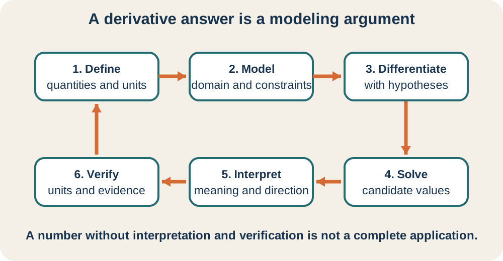
Begin by naming every quantity and its units. Identify the independent variable and the quantities that depend on it. State the physical or mathematical domain before differentiating. Translate verbal constraints into equations or inequalities. These definitions prevent a correct calculation from answering the wrong question.

Next, select the theorem that connects the model to the requested information. A derivative sign can establish increase or decrease, while a sign change can classify a local extremum. The Extreme Value Theorem supports absolute optimization on a closed interval. The Mean Value Theorem connects average and instantaneous rates. Related-rate problems use the chain rule after a geometric relationship has been established.

Finish by interpreting and verifying the result. Attach units and state whether the quantity increases, decreases, maximizes, or minimizes. Reject candidates outside the feasible domain. Check signs, dimensions, endpoint behavior, and approximate scale. A bare number is not a complete application because it does not communicate why the answer belongs to the model.

Translate position into velocity and acceleration

Let $s(t)$ denote position as a function of time. Velocity is $v(t)=s'(t)$, so it measures signed position change per unit time. Acceleration is $a(t)=v'(t)=s''(t)$, so it measures signed velocity change per unit time. The prime symbol indicates differentiation with respect to the displayed input $t$. If position uses meters and time uses seconds, velocity uses meters per second and acceleration uses meters per second squared.

Direction comes from the sign of velocity. Positive velocity means motion in the positive coordinate direction, while negative velocity means motion in the negative direction. An object is stationary when $v(t)=0$. A stationary time is only a candidate for reversal. Reversal occurs only when velocity changes sign across that time.

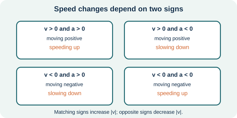
Speed is the magnitude $|v(t)|$, not the signed velocity itself. An object speeds up when velocity and acceleration share a sign because acceleration pushes velocity farther from zero. It slows down when their signs differ because acceleration pushes velocity toward zero. This criterion works for motion in either coordinate direction. Reading both signs prevents the common mistake of treating positive acceleration as automatic speeding up.

Distinguish displacement from total distance

Displacement on $[a,b]$ is $s(b)-s(a)$. It measures net position change and can be positive, negative, or zero. Total distance measures all ground traveled and cannot be negative. Compute it by splitting the interval wherever velocity changes sign. Add the absolute position changes over the resulting intervals.

Consider $s(t)=t^2-4t$ meters on $0\le t\le5$ seconds. Velocity is $v(t)=2t-4$ meters per second, which is zero at $t=2$ seconds. Its sign changes from negative to positive there, so the object reverses. Displacement is $s(5)-s(0)=5$ meters. This value records only the net shift from start to finish.

For total distance, evaluate position at zero, two, and five seconds. Those positions are $0$ meters, $-4$ meters, and $5$ meters. The distance is $|-4\,\mathrm{m}-0\,\mathrm{m}|+|5\,\mathrm{m}-(-4\,\mathrm{m})|$. The result is $4$ meters plus $9$ meters, or $13$ meters. The difference between $5$ meters and $13$ meters is the motion that displacement cancels but distance retains.

Infer graph behavior from the first derivative

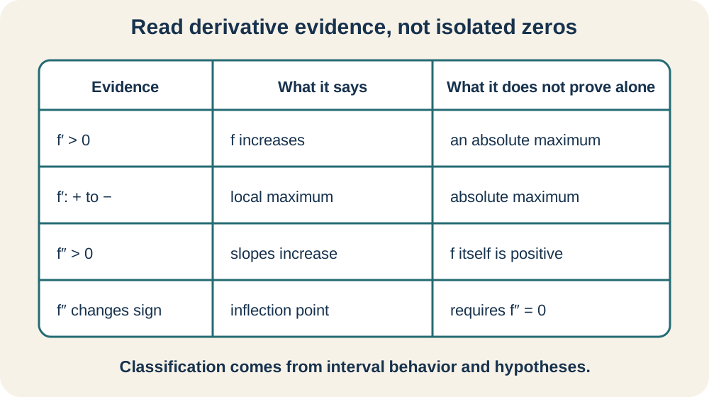
If $f'(x)>0$ throughout an interval, then $f$ increases there. If $f'(x)<0$, then $f$ decreases there. A critical number is an interior domain value where $f'(x)=0$ or where $f'(x)$ does not exist. Critical numbers organize the sign chart. They do not automatically represent maxima or minima.

The first derivative test classifies a local maximum when $f'$ changes from positive to negative. It classifies a local minimum when $f'$ changes from negative to positive. If the sign does not change, the critical number is neither kind of local extremum. Testing one representative point in each interval is often enough when the derivative’s sign structure is known. Record the intervals before assigning the classification.

For $f(x)=x^3-3x^2$, the derivative is $f'(x)=3x(x-2)$. It is positive on $(-\infty,0)$, negative on $(0,2)$, and positive on $(2,\infty)$. Therefore $f$ has a local maximum at $x=0$ and a local minimum at $x=2$. These are local conclusions based on neighboring behavior. Absolute conclusions require comparison across the entire stated domain.

Use the second derivative to analyze concavity

The second derivative measures how the first derivative changes. If $f''(x)>0$, slopes increase and the graph is concave up. If $f''(x)<0$, slopes decrease and the graph is concave down. Concavity describes slope behavior rather than whether function values themselves are positive. A negative function can still be concave up.

An inflection point occurs where concavity actually changes. The equation $f''(c)=0$ only identifies a candidate. A sign chart or other argument must confirm opposite concavity on the two sides. The second derivative may also fail to exist at an inflection point. Classification depends on behavior, not on a single algebraic equality.

When $f'(c)=0$, the second derivative test can classify some critical points. If $f''(c)>0$, the locally concave-up graph has a local minimum at $c$. If $f''(c)<0$, the locally concave-down graph has a local maximum. If $f''(c)=0$ or is undefined, the test is inconclusive. Return to the first derivative test rather than declaring that no extremum exists.

Apply the Mean Value Theorem

Suppose $f$ is continuous on the closed interval $[a,b]$ and differentiable on the open interval $(a,b)$. The Mean Value Theorem guarantees at least one $c$ in $(a,b)$ such that $f'(c)=\frac{f(b)-f(a)}{b-a}$. The right side is the average rate of change across the interval. The left side is an instantaneous rate at an interior point. The theorem connects a secant slope to at least one parallel tangent slope.

For $f(x)=x^2$ on $[1,4]$, the average rate is $\frac{16-1}{4-1}=5$. The polynomial is continuous on the closed interval and differentiable inside it. Its derivative is $f'(x)=2x$. Solving $2c=5$ gives $c=2.5$. This value lies inside $(1,4)$, as the conclusion requires.

The hypotheses are not optional decoration. The function $f(x)=\frac{1}{x}$ on $[-1,1]$ is not continuous because it is undefined at zero. Its endpoint values give an average slope, but the theorem cannot guarantee the required interior derivative. Discontinuities can break the geometric connection between the secant and tangent. Always state both hypotheses before invoking the conclusion.

Find absolute extrema on a closed interval

The Extreme Value Theorem states that a continuous function on a closed interval attains an absolute maximum and an absolute minimum. Continuity, closedness, and boundedness of the interval are all part of the guarantee. The theorem establishes existence but does not locate the extrema. Derivatives generate interior candidates. Endpoints complete the candidate list.

Use the closed-interval method systematically. Find all interior points where $f'=0$ or $f'$ does not exist while $f$ does. Evaluate the original function at those points and at both endpoints. Compare the resulting output values rather than the inputs. The largest output is the absolute maximum and the smallest is the absolute minimum.

For $f(x)=x^2-4x+1$ on $[0,5]$, solve $f'(x)=2x-4=0$ to get $x=2$. Evaluate $f(0)=1$, $f(2)=-3$, and $f(5)=6$. The absolute minimum is $-3$ at $x=2$. The absolute maximum is $6$ at $x=5$. Ignoring endpoints would have missed the maximum even though the derivative work was correct.

Build and justify an optimization model

Optimization begins before differentiation. Define the objective quantity and the constraint relating the variables. Use the constraint to express the objective in one independent variable. Determine the feasible domain from geometry, units, and physical limitations. Only then differentiate to find candidates.

Suppose a rectangle has perimeter $40$ meters and one side has length $x$ meters. The other side is $20-x$ meters because $2x+2y=40$ meters implies $y=20-x$ meters. Area is $A(x)=x(20-x)$ square meters. The feasible closed interval is $0\le x\le20$ meters if degenerate endpoints are admitted for comparison. The derivative is $A'(x)=20-2x$ meters.

Solving $A'(x)=0$ gives $x=10$ meters. The corresponding other side is also $10$ meters, and the area is $100$ square meters. Both endpoint areas are zero square meters. Therefore the square gives the absolute maximum on the feasible interval. This conclusion uses the model, critical point, endpoints, and contextual interpretation together.

Construct and evaluate a linearization

Differentiability means a smooth function is locally well approximated by its tangent line. Near $x=a$, the linearization is $L(x)=f(a)+f'(a)(x-a)$. The value $f(a)$ anchors the line at the known point. The derivative $f'(a)$ supplies its slope. The difference $x-a$ measures the nearby input change.

Approximate $\sqrt{101}$ using $f(x)=\sqrt{x}$ near $a=100$. The known value is $f(100)=10$, and the derivative is $f'(x)=\frac{1}{2\sqrt{x}}$. Thus $f'(100)=\frac{1}{20}$. Substitution gives $L(101)=10+\frac{1}{20}(1)=10.05$. This is an approximation rather than an algebraic identity.

Curvature helps predict the error direction. The square-root function is concave down for positive inputs, so its tangent line lies above the nearby graph. The estimate therefore slightly exceeds the true value. Greater distance from the base point usually increases error. A useful report includes the base point, approximation, and qualitative error expectation.

Solve related-rate problems symbolically first

Related rates involve several quantities that change with a shared independent variable, usually time. Begin with an equation relating the quantities themselves. Differentiate that equation with respect to time using the chain rule. Keep changing variables symbolic during differentiation. Substitute the instant-specific measurements only afterward.

For a circle, area and radius satisfy $A=\pi r^2$. Differentiating with respect to time gives $\frac{dA}{dt}=2\pi r\frac{dr}{dt}$. The factor $\frac{dr}{dt}$ appears because radius depends on time. If radius grows at $0.50\,\frac{\mathrm{cm}}{\mathrm{s}}$ when $r=4.0$ centimeters, substitute those values after deriving the rate equation. The area then grows at $4\pi\,\frac{\mathrm{cm^2}}{\mathrm{s}}$.

Substituting radius too early would replace a changing quantity with one fixed number. Differentiation would then incorrectly treat it as constant and erase its rate. Units also verify the result because centimeters times centimeters per second gives square centimeters per second. The positive sign agrees with an expanding radius. Symbolic-first work preserves dependency and makes these checks visible.

Combine derivative evidence in one argument

Applications often require several derivative ideas at once. A graph-analysis problem may ask for increase, extrema, concavity, and inflection points. Build separate sign charts for $f'$ and $f''$ rather than mixing their roles. Use $f'$ for motion of the function and $f''$ for motion of its slopes. Combine conclusions only after each chart is correct.

For $f(x)=x^3-3x^2$, recall $f'(x)=3x(x-2)$ and compute $f''(x)=6(x-1)$. The first derivative gives a local maximum at zero and a local minimum at two. The second derivative is negative before one and positive after one. Therefore the graph has an inflection point at $x=1$. The three special inputs arise from different conditions and need not coincide.

Write conclusions in complete contextual language. Say that the function increases on specified intervals instead of merely writing plus signs. Say that concavity changes from down to up at the inflection point. Distinguish a local extremum from an absolute one. Precise language reveals whether the derivative evidence has actually been interpreted.

Practice, diagnose, and connect forward

Analyze $s(t)=t^2-6t$ meters on $0\le t\le7$ seconds. Compute velocity, locate any reversal, and distinguish displacement from total distance. Then decide where the object speeds up or slows down by comparing velocity and acceleration signs. Keep seconds and fractional motion units in every numerical statement. A diagram of the timeline can support the sign analysis.

Next, optimize a cylinder or enclosure by defining the objective and constraint before differentiating. State the feasible interval and compare endpoints with all interior candidates. Explain whether the derivative proves local or absolute behavior. Verify that the result has the correct dimensional units. If the model excludes material thickness or waste, identify that simplifying assumption.

Finally, approximate a nearby value by linearization and solve one geometric related-rate problem. For each, name the derivative’s meaning in words. Predict a sign or approximate size before calculating. Compare that prediction with the result. Integration will reverse local rate information into accumulated change, extending the same modeling discipline into the next calculus sequence.

Sources and further study

OpenStax Calculus, Volume 1 provides derivations and exercises for derivative applications. Its chapters treat motion, graph analysis, optimization, linearization, and related rates. Compare its worked solutions with the workflow used here. Identify where each solution defines a domain and verifies a conclusion. Reworking an example without viewing its algebra provides effective retrieval practice.

The AP Calculus AB course overview supplies curriculum alignment for these application categories. It emphasizes representations, justification, and contextual interpretation in addition to calculation. Use its topic sequence to locate prerequisites that need review. Pay attention to theorem hypotheses in free-response reasoning. A named theorem should always be paired with evidence that its assumptions hold.

Further study should connect these methods to definite integrals and differential equations. Derivatives describe instantaneous change, while integrals accumulate that change across intervals. Differential equations encode relationships among quantities and their derivatives. Make a concept map joining local behavior, accumulated behavior, and model constraints. This broader organization keeps applications from becoming an unrelated collection of tricks.