Derivative as a Limit

A derivative is a limit of average rates over shrinking nonzero intervals. It measures instantaneous change, tangent-line slope, and the coefficient of the best local linear approximation. The interval width is never set equal to zero inside the quotient because division by zero would be undefined. Instead, limits study what the quotient approaches as the width becomes arbitrarily small. This lesson connects the algebraic definition to geometry, motion, units, continuity, approximation error, and failure modes.

Learning objectives and the local-change question

By the end of this lesson, you will construct a difference quotient from two function values. You will evaluate derivative limits using algebra rather than direct division by zero. You will interpret derivatives as tangent slopes and instantaneous rates with units. You will connect differentiability to local linear approximation and continuity. You will also classify corners, cusps, vertical tangents, discontinuities, and oscillation as distinct failure modes.

Average rate describes change across an interval. If the interval is wide, the result blends behavior from many inputs. Instantaneous rate asks what remains when the interval is made arbitrarily narrow around one input. A limit makes this question precise. The derivative is therefore built from average change rather than invented as an unrelated operation.

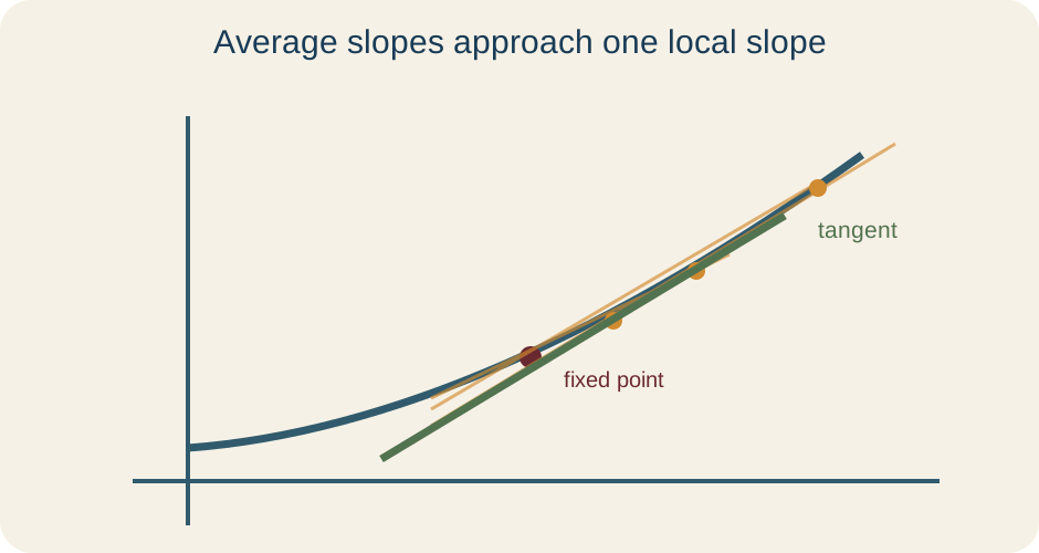
Geometry supplies the same progression. A secant line connects two points on a graph and has an average slope. As the second point approaches the first, secant slopes may approach one limiting value. The tangent line uses that limiting slope. The diagram below shows the moving secant and its limiting tangent without claiming the two points ever become distinct points at zero separation.

Construct the difference quotient

Fix an input $a$ and choose a nonzero increment $h$. The second input is $a+h$. The output change is $f(a+h)-f(a)$. The input change is $(a+h)-a=h$. Dividing gives the average rate $\frac{f(a+h)-f(a)}{h}$.

The numerator and denominator have distinct meanings. The numerator measures vertical output change. The denominator measures horizontal input change. Their quotient has output units per input unit. A sign indicates whether output rises or falls as input moves in the chosen direction.

The condition $h\ne0$ is essential. At zero, both sampled inputs coincide and the quotient would divide by zero. The derivative does not repair that undefined value by substitution. It asks whether nearby nonzero quotients approach a finite number. This distinction between value and limit is the conceptual heart of the definition.

Define the derivative precisely

If the limit exists and is finite, define $f'(a)=\lim_{h\to0}\frac{f(a+h)-f(a)}{h}$. The prime notation $f'(a)$ names the derivative value at input $a$. The arrow $h\to0$ means $h$ approaches zero through nonzero values from both sides. A two-sided limit requires agreement from positive and negative increments. The result is a number, not a new input interval.

An equivalent definition is $f'(a)=\lim_{x\to a}\frac{f(x)-f(a)}{x-a}$. Here $x$ is the moving second input. The denominator $x-a$ plays the same role as $h$. Substituting $x=a+h$ converts one form into the other. Choose the form best aligned with the algebra or data given.

The derivative function $f'(x)$ assigns a derivative value to every input where the defining limit exists. Do not confuse the function with one value $f'(a)$. A function may be differentiable on part of its domain and fail at isolated points. State the relevant input or interval. Domain is part of derivative information.

Derive the derivative of a square

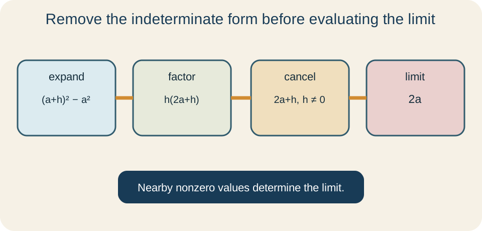
Let $f(x)=x^2$. At input $a$, the difference quotient is $\frac{(a+h)^2-a^2}{h}$. Expanding gives $\frac{a^2+2ah+h^2-a^2}{h}$. Combining terms yields $\frac{2ah+h^2}{h}$. Factoring the numerator gives $\frac{h(2a+h)}{h}$.

Because $h\ne0$ in the difference quotient, canceling the common factor is valid. The quotient becomes $2a+h$. Now the limit as $h\to0$ can be evaluated directly. It is $2a$. Therefore the derivative of $x^2$ at $a$ is $f'(a)=2a$.

The original zero-over-zero form was indeterminate, not an answer. Algebra revealed the nearby behavior that direct substitution concealed. Cancellation does not evaluate the quotient at zero. It produces an equivalent expression for every nonzero $h$ near zero. Limits depend on those nearby values, so the simplified form determines the limit.

Derive a linear-function result

Let $f(x)=mx+b$, where $m$ and $b$ are constants. The difference quotient is $\frac{m(a+h)+b-(ma+b)}{h}$. Distributing the subtraction leaves $\frac{mh}{h}$. For nonzero $h$, the quotient equals $m$. Its limit is therefore $m$.

This result agrees with line geometry. Every secant line on a nonvertical straight line has the same slope. Shrinking the interval does not change that slope. The constant $b$ shifts the graph vertically without changing rate. Thus the derivative of $mx+b$ is the constant $m$.

Units still matter. If $f$ is cost in dollars and $x$ is production in items, then $m$ has dollars-per-item units. The derivative reports marginal cost in the linear model. The intercept $b$ has dollar units. A derivative equal to $m$ is not unitless merely because it is constant.

Derive a reciprocal-function result

Let $f(x)=\frac{1}{x}$ and choose $a\ne0$. Also require $a+h\ne0$ for nearby quotient values. The difference quotient contains $\frac{1}{a+h}-\frac{1}{a}$. Combining these fractions gives $\frac{a-(a+h)}{a(a+h)}$. The numerator simplifies to $-h$.

Dividing the combined difference by $h$ gives $\frac{-h}{a(a+h)h}$. Cancel the nonzero factor $h$. The quotient becomes $-\frac{1}{a(a+h)}$. Taking $h\to0$ gives $-\frac{1}{a^2}$. Therefore $f'(a)=-\frac{1}{a^2}$ for $a\ne0$.

The original domain restriction survives differentiation. The formula $-\frac{1}{a^2}$ is also undefined at zero. Its negative sign matches the fact that $1/x$ decreases on each domain interval. The derivation uses common denominators before cancellation. Skipping that algebra is a common source of sign and denominator errors.

Interpret instantaneous velocity with units

Let position be $s(t)=\left(3.0\,\frac{\mathrm{m}}{\mathrm{s}^2}\right)t^2$. The average velocity from $t$ to $t+h$ is $\frac{s(t+h)-s(t)}{h}$. Its limit as $h\to0$ is instantaneous velocity. The derivative is $s'(t)=\left(6.0\,\frac{\mathrm{m}}{\mathrm{s}^2}\right)t$. Time remains the input variable.

At $t=2.0\,\mathrm{s}$, velocity is $12.0\,\frac{\mathrm{m}}{\mathrm{s}}$. The coefficient’s acceleration-like units multiply time and produce velocity units. Position change divided by time change also yields meters per second. Two independent unit routes agree. That agreement checks the derivative interpretation.

Instantaneous velocity is not distance divided by zero time. It is the limit of displacement-per-time ratios over nonzero durations. A negative velocity indicates motion in the chosen negative direction. Zero velocity means no instantaneous position change at that moment. It does not necessarily mean the object remains still over a surrounding interval.

Connect derivatives to tangent lines

If $f'(a)$ exists, the tangent line at $(a,f(a))$ is $L(x)=f(a)+f'(a)(x-a)$. The coefficient $f'(a)$ is the slope. The expression $x-a$ is horizontal displacement from the tangent point. Multiplying slope by horizontal displacement predicts vertical change. Adding $f(a)$ anchors the line at the correct point.

For $f(x)=x^2$ at $a=3$, the derivative is six and the point is $(3,9)$. The tangent line is $L(x)=9+6(x-3)$. In point-slope form it is $y-9=6(x-3)$. Substituting $x=3$ returns $y=9$. Its slope matches the derivative limit.

A tangent line is not defined merely as a line that touches once. A tangent can cross the graph, and a secant can touch at more than one point. The limiting-slope definition is more reliable. Local behavior, not a global count of intersections, determines tangency. This distinction matters for inflection points and oscillating graphs.

Understand local linearity

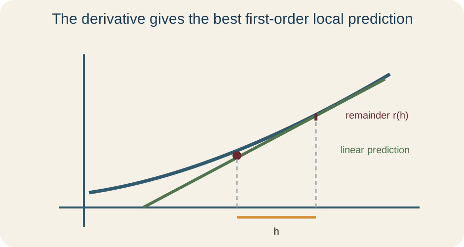
Differentiability means more than having a tangent slope. For small $h$, $f(a+h)=f(a)+f'(a)h+r(h)$, where the remainder satisfies $\lim_{h\to0}\frac{r(h)}{h}=0$. The term $f'(a)h$ is the predicted output change. The remainder is the prediction error. Its size becomes negligible compared with $h$.

The local linear approximation is $f(a+h)\approx f(a)+f'(a)h$. It replaces the function near $a$ with its tangent line. The approximation generally worsens as $|h|$ grows. It is local rather than global. A derivative therefore measures both rate and best first-order approximation.

For $f(x)=\sqrt{x}$ near nine, $f(9)=3$ and $f'(9)=\frac{1}{6}$. With $h=0.12$, the approximation gives $\sqrt{9.12}\approx3+\frac{0.12}{6}=3.02$. The square-root graph is concave down, so its tangent lies slightly above the graph nearby. The estimate should therefore be a slight overestimate. Concavity helps interpret the direction of error.

Prove differentiability implies continuity

Assume $f'(a)$ exists and is finite. For $x\ne a$, write $f(x)-f(a)=\frac{f(x)-f(a)}{x-a}(x-a)$. As $x\to a$, the quotient approaches $f'(a)$. The factor $x-a$ approaches zero. Their product approaches zero.

Thus $f(x)-f(a)\to0$, which means $f(x)\to f(a)$. This is continuity at $a$. Differentiability therefore implies continuity. A discontinuous function cannot be differentiable at the discontinuity. Continuity is a necessary condition for finite differentiability.

The converse is false. The function $f(x)=|x|$ is continuous at zero. Its right-hand difference quotients approach one, while its left-hand quotients approach negative one. The two-sided derivative limit does not exist. Continuity alone does not guarantee a single tangent slope.

Analyze one-sided derivatives

The right derivative uses $h\to0^+$, meaning positive increments. The left derivative uses $h\to0^-$, meaning negative increments. A finite two-sided derivative exists only when both one-sided derivatives exist and are equal. One-sided derivatives are especially useful at corners and domain endpoints. State which direction is being considered.

For $f(x)=|x|$ at zero, positive $h$ gives quotient $\frac{|h|-0}{h}=1$. Negative $h$ gives quotient $\frac{-h}{h}=-1$. Because the limits differ, no two-sided derivative exists. The graph has a corner. Its continuity does not resolve the conflicting slopes.

At an endpoint, a context may use only one side. If time begins at zero, a right derivative can describe the initial rate. Standard differentiability on an open interval uses two-sided limits at interior points. Do not invent nonexistent inputs outside the domain. Match the derivative definition to the domain and question.

Classify derivative failure modes

A discontinuity prevents differentiability because differentiability implies continuity. A corner has unequal finite one-sided slopes. A cusp has one-sided slopes of opposite infinite signs. A vertical tangent has slopes whose magnitudes grow without bound with compatible direction. Standard finite differentiability fails in all four cases.

Oscillation can also prevent a limiting slope. Difference quotients may keep changing without settling as the interval shrinks. A graph can remain continuous while its local slopes oscillate. Visual smoothness at ordinary scale may hide this behavior. The limit definition is the final test.

Naming the failure mode provides more information than saying “not differentiable.” Compare one-sided limits, check continuity, and inspect whether slope magnitude remains finite. A vertical tangent can still have a meaningful geometric tangent line even though the derivative is not finite. A corner has two competing tangent directions. An oscillatory failure may have no stable tangent direction at all. Each case calls for precise language.

Approximate derivatives from data

When a formula is unavailable, nearby data can approximate a derivative. A forward difference uses $\frac{f(a+h)-f(a)}{h}$. A backward difference uses $\frac{f(a)-f(a-h)}{h}$. A centered difference uses $\frac{f(a+h)-f(a-h)}{2h}$. Centering often balances first-order errors for smooth functions.

Smaller $h$ does not guarantee unlimited numerical improvement. Measurement noise becomes magnified when divided by a very small interval. Computer roundoff can also cause subtractive cancellation. Choose a scale that balances local approximation with data quality. Report uncertainty and units.

A table of secant slopes can suggest convergence. Use positive and negative increments when a two-sided derivative is claimed. Values approaching the same number support differentiability but do not prove it from finitely many samples. A symbolic limit or theorem provides stronger evidence. Numerical work remains valuable for exploration and checking.

Diagnose common mistakes

Substituting $h=0$ into the original quotient creates division by zero. Canceling $h$ before showing it is a common factor is invalid. Expanding $(a+h)^2$ without the cross term changes the function. Forgetting the subtraction parentheses changes the numerator. Each error disrupts the limit structure.

The derivative is not always the function value divided by the input. It is not merely the slope from the origin. It is not guaranteed by continuity. It is not automatically finite at a vertical tangent. The definition decides each case.

Units offer a fast check. A temperature derivative with respect to time must have temperature-per-time units. The increment $f'(a)h$ must have output units. A tangent equation must pass through $(a,f(a))$. These checks complement the formal limit calculation.

Guided practice and connection forward

Use the definition for $f(x)=3x+5$. The difference quotient simplifies to $\frac{3h}{h}=3$ for $h\ne0$. Its limit is three. Therefore $f'(a)=3$ for every real $a$. This matches the line’s constant slope.

For $f(x)=|x-2|$, analyze the derivative at two. Positive increments produce slope one, while negative increments produce slope negative one. The one-sided limits differ. Therefore the graph has a corner and is not differentiable at two. The function remains continuous there.

For independent synthesis, use the limit definition to find the derivative of $f(x)=\frac{1}{x}$ at $a=2$. State every domain restriction and common-denominator step. Then interpret $T'(3\,\mathrm{min})=-0.8\,\frac{{}^\circ\mathrm{C}}{\mathrm{min}}$ in words. Include the meaning of the negative sign and the units. Basic differentiation rules will compress these repeated limit arguments while preserving the same local-change meaning.