Basic Differentiation Rules

Differentiation rules are reusable consequences of the limit definition. They make computation efficient without changing the derivative’s meaning as instantaneous rate and local linear coefficient. Every rule has a structural scope, so choosing the rule is as important as carrying it out. Domain restrictions remain attached to the original function even when a derivative formula looks broader. This lesson derives the foundational rules, explains their notation, and verifies results with units, signs, degrees, and numerical difference quotients.

Learning objectives and the role of rules

By the end of this lesson, you will derive constant, constant-multiple, sum, and positive-integer power rules from limits. You will extend the power rule carefully to negative and fractional exponents. You will differentiate polynomial, exponential, sine, and cosine functions. You will choose a rule from the expression’s outermost structure. You will also state derivative domains and interpret results with appropriate units.

A differentiation rule compresses a limit argument that has already been justified. Using a rule is not abandoning rigor when its hypotheses are satisfied. It is citing a theorem instead of repeating its proof. The derivative still measures the limit of a difference quotient. Efficient notation lets attention shift from repeated algebra to structure and interpretation.

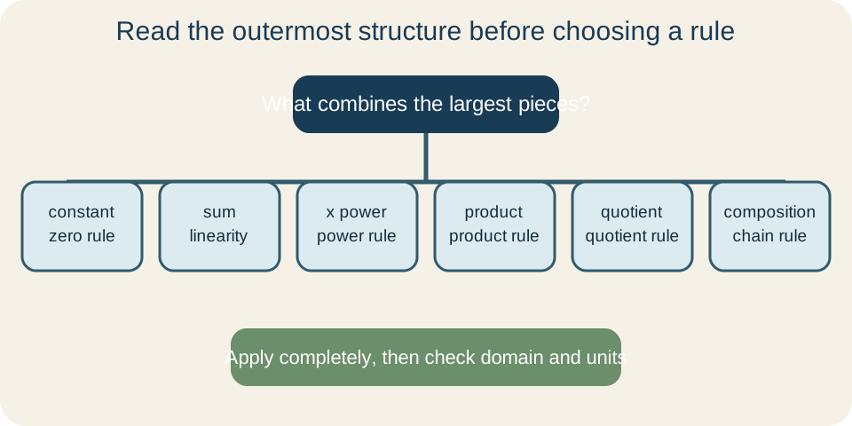
Rules do not all distribute across all operations. Linearity handles finite sums and constant multiples. Products, quotients, and compositions require additional rules because their parts change together. The roadmap below separates these outer structures. Accurate classification prevents an appealing but invalid shortcut.

Derive the constant rule

Let $f(x)=c$, where $c$ is constant. The difference quotient is $\frac{c-c}{h}$. Its numerator is zero for every nonzero $h$. Therefore the quotient is zero. Its limit is also zero.

The constant rule is $\frac{d}{dx}c=0$. The operator $\frac{d}{dx}$ means differentiate with respect to $x$. A constant output has no local change as $x$ varies. Its graph is horizontal. A horizontal line has slope zero.

Units reinforce the meaning. If $c$ is a fixed volume in liters and $x$ is time in seconds, the derivative is zero liters per second. The number zero still belongs to a rate quantity. Writing no units can hide the variable of differentiation. State units when the context supplies them.

Derive constant-multiple and sum rules

Let $F(x)=af(x)$ for constant $a$. Its difference quotient is $a\frac{f(x+h)-f(x)}{h}$. A constant can pass through the limit when the derivative exists. Therefore $F'(x)=af'(x)$. Scaling outputs by $a$ scales every output change by $a$.

For $F(x)=f(x)+g(x)$, split the numerator into the change in $f$ plus the change in $g$. The quotient becomes the sum of two difference quotients. Limit laws give $(f+g)'=f'+g'$. Subtraction follows by using constant negative one. Finite sums can therefore be differentiated term by term.

Together these statements express linearity: $\frac{d}{dx}[af(x)+bg(x)]=af'(x)+bg'(x)$. The constants $a$ and $b$ do not depend on $x$. Linearity does not say $(fg)'=f'g'$ or $[f(g(x))]'=f'(g'(x))$. Multiplicative and nested structures are not linear combinations. Their derivatives require rules that account for interaction between changing factors.

Derive the positive-integer power rule

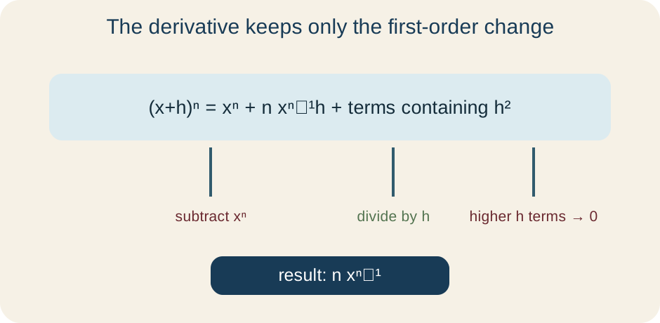
For $f(x)=x^n$ with positive integer $n$, begin with $\frac{(x+h)^n-x^n}{h}$. The binomial theorem expands $(x+h)^n$. Its first two terms are $x^n+nx^{n-1}h$. Every later term contains at least $h^2$. Subtracting $x^n$ removes the constant-order term.

After division by nonzero $h$, the leading term is $nx^{n-1}$. Every remaining term still contains at least one factor of $h$. As $h\to0$, those terms vanish. Therefore $\frac{d}{dx}x^n=nx^{n-1}$. The old exponent becomes a coefficient and the exponent decreases by one.

The derivation explains both changes in the rule. There are $n$ first-order ways for one factor in the product $x^n$ to contribute an increment. Removing one increment factor leaves $n-1$ factors of $x$. The rule is not a symbol-moving trick. It records the first-order part of the binomial expansion.

Apply the power rule to polynomials

A polynomial is a finite sum of constant multiples of nonnegative integer powers. Linearity and the power rule therefore apply term by term. For $f(x)=4x^5-3x^2+7x-9$, differentiate each term. The result is $f'(x)=20x^4-6x+7$. The constant term disappears.

At $x=1$, the derivative value is $20-6+7=21$. This number is the tangent slope and instantaneous output rate per input unit. It is not the function value. The original value is $f(1)=4-3+7-9=-1$. Function value and derivative value answer different questions.

A nonconstant polynomial of degree $n$ normally has derivative degree $n-1$. This observation checks the leading behavior. Leading-term cancellation can lower the degree further only after like terms are combined. A proposed derivative with higher degree than the original polynomial is immediately suspicious. Degree is a useful diagnostic, not the derivation itself.

Extend the rule to negative exponents

Negative exponents represent reciprocals. For $x\ne0$, $x^{-m}=\frac{1}{x^m}$. The generalized power rule gives $\frac{d}{dx}x^{-m}=-mx^{-m-1}$. This extension can be proved using quotient rules or other limit arguments. The original exclusion $x\ne0$ remains.

Differentiate $5x^4-2x^{-1}+8$. The first term gives $20x^3$. The second gives $2x^{-2}$ because $(-2)(-1)=2$. The constant gives zero. Thus the derivative is $20x^3+\frac{2}{x^2}$ for $x\ne0$.

Sign deserves attention. The derivative of $x^{-1}=\frac{1}{x}$ is $-x^{-2}$, which is negative on both domain intervals. This agrees with the reciprocal function decreasing on each interval. A sign check catches a lost negative coefficient. Domain and qualitative behavior support the calculation.

Apply the rule to fractional exponents

Fractional powers represent roots under real-domain conventions. The function $x^{1/2}=\sqrt{x}$ has real domain $x\ge0$. For $x>0$, the power rule gives $\frac{d}{dx}x^{1/2}=\frac{1}{2}x^{-1/2}=\frac{1}{2\sqrt{x}}$. The derivative formula requires a positive input. It becomes unbounded as $x\to0^+$.

Continuity at zero does not guarantee finite differentiability there. The right difference quotient for $\sqrt{x}$ at zero is $\frac{\sqrt{h}}{h}=\frac{1}{\sqrt{h}}$. It grows without bound as $h\to0^+$. The function also lacks real inputs to the left of zero. Therefore the standard two-sided finite derivative does not exist at zero.

Other rational exponents require domain analysis. Odd roots may accept negative inputs, while even roots do not. Negative fractional exponents add denominator restrictions. State an interval where the function is real and differentiable. Do not let a formal power-rule expression silently enlarge the domain.

Differentiate exponential functions

The natural exponential function satisfies $\frac{d}{dx}e^x=e^x$. The number $e$ is approximately $2.71828$. It is distinguished by having instantaneous relative growth rate one. The derivative equals the original output at every input. This self-reproduction makes $e^x$ central in calculus.

For a positive base $a$, $\frac{d}{dx}a^x=a^x\ln a$. The symbol $\ln a$ is the natural logarithm of the base. The limit $\lim_{h\to0}\frac{a^h-1}{h}=\ln a$ produces that factor. When $a=e$, $\ln e=1$. The formula reduces to the natural exponential rule.

If $0<a<1$, then $\ln a<0$, so $a^x$ decreases. If $a>1$, then $\ln a>0$, so it increases. The derivative sign matches graph behavior. A base must be positive for a real-valued exponential across all real inputs. Nested exponents such as $e^{kx}$ require the chain rule developed later.

Establish sine and cosine derivatives

Trigonometric derivative rules use radian measure. The foundational limits are $\lim_{h\to0}\frac{\sin h}{h}=1$ and $\lim_{h\to0}\frac{\cos h-1}{h}=0$. Angle-addition identities then transform the difference quotients. The results are $\frac{d}{dx}\sin x=\cos x$ and $\frac{d}{dx}\cos x=-\sin x$. The negative sign reflects cosine’s local direction.

Radians are essential because they relate arc length directly to radius. In degree measure, conversion factors appear. A formula copied from radian calculus into a degree-input model is incomplete. State the angle unit when differentiation has a physical or computational context. Standard calculus notation assumes radians unless stated otherwise.

Graph checks support the signs. Sine increases most rapidly at zero, and $\cos0=1$. Cosine has horizontal slope at zero, and $-\sin0=0$. Near $\frac{\pi}{2}$, cosine is decreasing and $-\sin\frac{\pi}{2}=-1$. These values align with the derivative formulas.

Choose rules from outermost structure

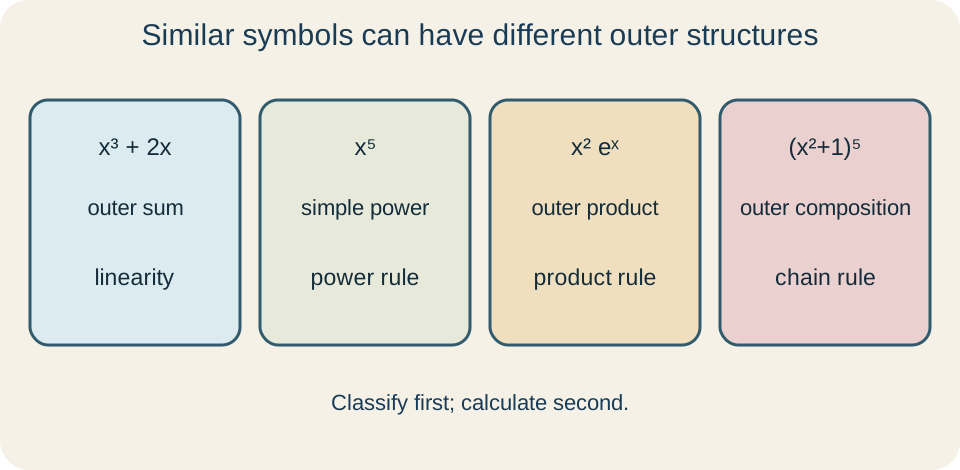
Before differentiating, identify the expression’s outermost operation. A finite sum calls for linearity. A single power of $x$ calls for the power rule. A product of varying functions calls for the product rule. A nested function calls for the chain rule.

The expression $(x^2+1)^5$ is a fifth power, but its base is not simply $x$. The inner quantity also changes with $x$. Writing $5(x^2+1)^4$ omits that inner rate. The chain rule supplies the missing factor. Do not apply the basic power rule as though a composite base were the independent variable.

Rewriting can reveal simpler structure. A square root may be written as a fractional power. A reciprocal may be written with a negative exponent. A polynomial should be expanded or combined before termwise differentiation when that reduces complexity. Preserve domain restrictions during every rewrite.

Preserve derivative domains

The derivative exists only where the original function is defined and differentiable. A simplified derivative formula cannot restore an excluded input. For $g(x)=3\sqrt{x}-\frac{2}{x}$, the original real domain is $x>0$. Both the root and reciprocal restrictions combine. The derivative must be reported on that domain.

Rewrite $g(x)=3x^{1/2}-2x^{-1}$. Differentiating gives $g'(x)=\frac{3}{2}x^{-1/2}+2x^{-2}$. In horizontal-fraction notation, this is $\frac{3}{2\sqrt{x}}+\frac{2}{x^2}$. Both terms are defined for $x>0$. That is the derivative’s inherited domain.

An absolute-value function illustrates another limitation. A formula may be defined and continuous at a corner but not differentiable there. A piecewise derivative must exclude the corner unless one-sided slopes agree. Rule application within pieces does not settle their boundary. Check transition points separately with one-sided derivatives.

Interpret derivatives with units

If $Q(t)$ is measured in liters and $t$ in seconds, then $Q'(t)$ has liters-per-second units. A negative derivative means the quantity is locally decreasing. It does not mean the quantity itself is negative. Function value and rate have different units and meanings. Always interpret both separately.

Suppose $s(t)$ is position in meters. Then $s'(t)$ is velocity in meters per second. Differentiating again gives acceleration in meters per second squared. Each derivative divides by another time unit. Dimensional analysis tracks this hierarchy.

In economics, if $C(q)$ is cost in dollars and $q$ is units produced, then $C'(q)$ has dollars-per-unit units. It approximates the additional cost of a small production increase near $q$. A derivative at a discrete count is a continuous-model approximation. State that assumption. Context determines how the local rate should be used.

Verify derivatives efficiently

Use a small centered difference $\frac{f(x+h)-f(x-h)}{2h}$ to approximate a derivative numerically. Compare it with the symbolic formula at a permitted input. Several moderate values of $h$ are more informative than one extremely small value. Roundoff and measurement noise can dominate when $h$ is too small. Numerical agreement supports but does not prove the rule application.

Check qualitative behavior. If a graph increases on an interval, a proposed derivative that is negative everywhere there is inconsistent. A local maximum often has derivative zero when differentiability holds. Exponential derivative signs should match their bases. Polynomial degree should usually decrease by one.

Check units and domains. The derivative’s units must be output units per input unit. Every evaluation input must belong to the original derivative domain. A formula that divides by zero is invalid there. Independent checks catch errors that repeated symbolic inspection may miss.

Diagnose common mistakes

The power rule multiplies by the old exponent before subtracting one from it. Doing only one of those operations is incomplete. The rule does not distribute through a sum inside a power. Linearity applies to sums of functions, not products of their derivatives. Structure must be read first.

Do not use degree-mode trigonometric formulas without a conversion factor. Do not drop a negative sign from the cosine derivative. Do not claim a derivative formula proves differentiability at every displayed input. Do not ignore root and denominator restrictions. Each rule carries hypotheses.

Do not omit contextual units. Do not confuse $f'(a)$ with $f(a)$. Do not substitute values before differentiating a time-dependent relationship in later related-rate work. A clear workflow names the rule, applies it, simplifies, records domain, and interprets. Verification completes the solution.

Guided practice and connection forward

Differentiate $3e^x-4\cos x$. Linearity gives three times the derivative of $e^x$ minus four times the derivative of cosine. The result is $3e^x+4\sin x$. The plus sign arises because the cosine derivative already contains a negative sign. The real domain is all real numbers.

Find the slope of $f(x)=\sqrt{x}$ at four. For positive $x$, $f'(x)=\frac{1}{2\sqrt{x}}$. Evaluating gives $f'(4)=\frac{1}{4}$. The derivative is finite because four is inside the positive domain. If $x$ had length units, the resulting unit interpretation would require the function’s own units.

For independent synthesis, differentiate $5x^4-2x^{-1}+8$ and state its domain. Then differentiate $2^x+5\sin x$, explaining the factor $\ln2$ and the radian assumption. Finally, diagnose why $5(x^2+1)^4$ is incomplete as the derivative of $(x^2+1)^5$. Product, quotient, and chain rules will extend these foundations to simultaneous and nested change. Preserve your written reasoning so that those later rules can be compared with the linear rules learned here.