Average Rate of Change

Average rate of change measures how much an output changes per unit change in its input across a specified interval. It extends the familiar slope of a line to functions whose steepness varies from place to place. The calculation uses only endpoint values, yet its meaning connects algebra, graphs, tables, units, and context. This interval-based idea is foundational because calculus later asks what happens as the interval becomes arbitrarily small. A learner who can explain the average rate clearly is prepared to understand the derivative as more than a formula.

Learning objectives and the change-per-change habit

By the end of this lesson, you will calculate average rates from formulas, tables, graphs, and verbal descriptions. You will interpret the difference quotient as a ratio of output change to input change and as the slope of a secant line. You will preserve units, analyze signs, and explain why the result depends on the chosen interval. You will distinguish net change from total variation and average rate from instantaneous rate. You will also estimate, verify, and communicate rates in context.

The central habit is to identify two changes before dividing. The numerator must be final output minus initial output, and the denominator must be final input minus initial input. Both differences must follow the same endpoint order. The quotient then answers how much output change occurred for each one unit of input change on average. Writing labels beside the differences prevents a purely mechanical substitution.

Average rate is not the same as the average of two output values. The arithmetic mean $\frac{f(a)+f(b)}{2}$ describes a central output level, while the average rate $\frac{f(b)-f(a)}{b-a}$ describes change per input. These quantities generally have different units and answer different questions. A position average may be measured in meters, while average velocity is measured in meters per second. Units reveal the conceptual distinction immediately.

Build the difference quotient from endpoint change

For a function $f$ on endpoints $a$ and $b$ with $a\ne b$, the average rate of change is $\frac{f(b)-f(a)}{b-a}$. The value $f(a)$ is the initial output and $f(b)$ is the final output when the interval is traversed from $a$ to $b$. The numerator $f(b)-f(a)$ is written $\Delta f$, where the Greek capital delta denotes finite change. The denominator $b-a$ is written $\Delta x$ when the input is $x$. Thus the quotient may also be written $\frac{\Delta f}{\Delta x}$.

The horizontal fraction bar groups each complete difference. Parentheses around function evaluations clarify that the subtraction occurs after evaluation. The requirement $a\ne b$ ensures the input change is nonzero. Dividing by zero would not produce a finite interval rate. Domain restrictions are part of the definition, not an optional technical note.

Reversing both endpoint orders leaves the rate unchanged because $\frac{f(a)-f(b)}{a-b}=\frac{-[f(b)-f(a)]}{-(b-a)}$. The two negative signs cancel. Reversing only one difference changes the sign and creates an inconsistent direction convention. Choose initial and final endpoints, then use that order in both numerator and denominator. This orientation rule is especially important when $b<a$.

Interpret the quotient as a secant slope

The points $(a,f(a))$ and $(b,f(b))$ lie on the graph of $f$. The line through those two points is a secant line. Its vertical change is $f(b)-f(a)$ and its horizontal change is $b-a$. Therefore its slope is exactly the average rate of change. The algebraic quotient and geometric secant slope describe the same quantity.

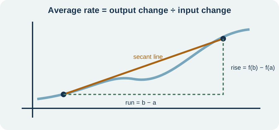
On a straight-line function, every secant slope equals the line’s constant slope. On a nonlinear function, different endpoint pairs generally produce different secant slopes. The secant line summarizes net change over one chosen interval rather than reproducing every detail of the curve. It may cross the graph, lie above it, or lie below it. Its role is endpoint comparison, not perfect local fit.

The sign of the secant slope gives net direction. A positive rate means the final output exceeds the initial output when the input increases from $a$ to $b$. A negative rate means the final output is smaller. A zero rate means the endpoint outputs are equal. None of these signs alone determines what happened between the endpoints.

Calculate from a formula in an auditable sequence

Suppose $f(x)=3x^2-x$ and the interval is $[1,4]$. Evaluate endpoints separately: $f(1)=3(1)^2-1=2$ and $f(4)=3(4)^2-4=44$. The output change is $44-2=42$, and the input change is $4-1=3$. Therefore the average rate is $\frac{42}{3}=14$. Keeping endpoint calculations separate makes substitution errors visible.

The answer’s units depend on what $x$ and $f(x)$ represent. If $x$ is measured in seconds and $f(x)$ in meters, then the rate is $14\ \frac{\mathrm m}{\mathrm s}$. If both quantities are dimensionless, the rate is dimensionless. If $f$ is cost in dollars and $x$ is quantity in items, the rate is dollars per item. A bare number is an incomplete applied interpretation.

Verification begins with estimation. Over the interval, the output rises by about forty units while the input rises by three, so a rate near thirteen or fourteen is plausible. A negative result would contradict the endpoint comparison. Substituting the secant line formula $L(x)=f(a)+m(x-a)$ with $m=14$ should produce both endpoint outputs. Multiple checks support the arithmetic and the interpretation.

Calculate from a table without inventing missing behavior

A table supplies sampled input-output pairs rather than a complete formula. To find an average rate on an interval whose endpoints appear in the table, subtract the corresponding outputs and divide by the input difference. Intermediate rows are not required for the endpoint quotient. They may nevertheless reveal whether behavior inside the interval is smooth, erratic, or nonmonotonic. The rate remains a summary of endpoints.

Suppose a population table shows $8{,}200$ people in year zero and $7{,}600$ people in year five. The net change is $7{,}600-8{,}200=-600$ people. The time change is $5.0\ \mathrm{yr}-0.0\ \mathrm{yr}=5.0\ \mathrm{yr}$. The average rate is $\frac{-600\ \mathrm{people}}{5.0\ \mathrm{yr}}=-120\ \frac{\mathrm{people}}{\mathrm{yr}}$. The negative sign indicates an average net decrease of 120 people per year.

This result does not prove the population declined by exactly 120 people during each individual year. It also does not reveal births, deaths, arrivals, or departures separately. Several different histories can share the same endpoint change. The word average refers to distributing the net change evenly over the input interval. State that limitation whenever the internal process matters.

Read a rate from a graph with scale awareness

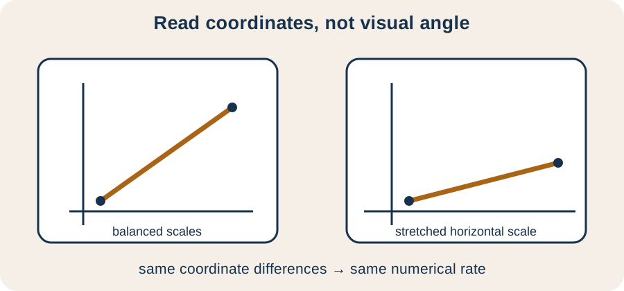
When a graph is the only representation, read approximate endpoint coordinates from the axes. Mark the two graph points, draw or imagine their secant, and calculate rise over run using the axis scales. A square on the horizontal axis may represent a different quantity from a square on the vertical axis. Visual angle alone cannot determine numerical slope. Axis labels and units control the calculation.

The diagram below separates graph steepness from plotting appearance. Two graphs can show the same function with different axis scales and make the curve look steeper or flatter. The numerical average rate remains unchanged when the coordinates are read correctly. Conversely, equal-looking angles on graphs with different scales can represent different rates. Never report slope from appearance without reading values.

Graph readings have limited precision. If each endpoint coordinate is estimated, the resulting differences inherit uncertainty. Reporting many decimal places suggests accuracy the graph does not support. Use approximately equal notation when values are read visually. A careful answer states both the estimated rate and the interval used.

Track units as a ratio of output to input

The units of average rate are output units divided by input units. If position is measured in meters and time in seconds, the quotient has units $\frac{\mathrm m}{\mathrm s}$. If temperature is degrees Celsius and height is meters, the rate has units $\frac{\mathrm{^{\circ}C}}{\mathrm m}$. The horizontal fraction makes the “per” relationship explicit. Units belong on intermediate differences as well as the final answer.

Consider position $s(t)=(2.0\ \frac{\mathrm m}{\mathrm{s^2}})t^2$ from $t=1.0\ \mathrm s$ to $t=4.0\ \mathrm s$. The endpoint positions are $2.0\ \mathrm m$ and $32\ \mathrm m$. Average velocity is $\frac{32\ \mathrm m-2.0\ \mathrm m}{4.0\ \mathrm s-1.0\ \mathrm s}=10\ \frac{\mathrm m}{\mathrm s}$. The coefficient’s units ensure that multiplying by $t^2$ produces meters. Every term remains dimensionally consistent.

Conversions must occur before subtracting incompatible measurements. A time interval mixing minutes and seconds should be expressed in one unit. A temperature difference may be measured in degrees Celsius even though absolute temperatures require care in other formulas. Unit cancellation should be displayed rather than assumed. Dimensional analysis can detect a swapped numerator and denominator.

Separate net change from total change

Average rate uses net output change $f(b)-f(a)$. If the function rises and later falls, opposite changes can cancel. A zero average rate means only that endpoint outputs match. It does not mean the function stayed constant or that no activity occurred. Net displacement and total distance provide a familiar example of this distinction.

Suppose a runner moves $100\ \mathrm m$ east and then $100\ \mathrm m$ west in $40\ \mathrm s$. Net displacement is zero, so average velocity is $0\ \frac{\mathrm m}{\mathrm s}$. Total distance is $200\ \mathrm m$, so average speed is $\frac{200\ \mathrm m}{40\ \mathrm s}=5.0\ \frac{\mathrm m}{\mathrm s}$. Velocity is based on directed displacement, while speed is based on accumulated distance. The two averages answer different questions.

A function can have zero average rate while possessing large positive and negative local rates. The secant line between equal endpoint heights is horizontal, even if the graph forms a tall arch between them. Endpoint summaries intentionally discard internal variation. If total change matters, another quantity must be computed. Choose the measure that matches the question rather than forcing the difference quotient to answer everything.

Understand interval dependence for nonlinear functions

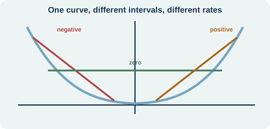
For $f(x)=x^2$, the average rate on $[a,b]$ is $\frac{b^2-a^2}{b-a}$. Factoring the numerator gives $\frac{(b-a)(b+a)}{b-a}=a+b$ when $a\ne b$. The rate therefore depends on both endpoints. A nonlinear function has no single global slope. Different intervals sample different parts of its changing steepness.

On $[0,2]$, the rate is $0+2=2$. On $[2,4]$, it is $2+4=6$. On $[-2,2]$, it is zero because the endpoint outputs are both four. These values are all correct for their respective intervals. Reporting an average rate without its interval is incomplete.

For a linear function $f(x)=mx+c$, the quotient simplifies to $m$ on every nonzero interval. This interval independence characterizes constant rate of change. The intercept $c$ cancels because it shifts both endpoint outputs equally. Nonlinear functions can have equal rates on some different intervals, but not necessarily all. Comparing intervals helps distinguish local behavior from a global linear model.

Interpret sign without assuming monotonicity

A positive average rate indicates net increase over the chosen orientation. It does not prove the function increased at every intermediate point. A graph may rise, fall, and rise again while ending above its start. Similarly, a negative average rate allows temporary increases. The quotient knows only the two endpoint values.

Monotonicity is a stronger property. A function is increasing on an interval when larger inputs consistently produce no smaller outputs under the chosen definition. Establishing monotonicity requires information across the interval, not just at its ends. A graph, formula, or derivative may provide that evidence. One secant slope cannot prove it.

The same caution applies in context. A positive average annual revenue change does not imply revenue increased every year. A negative average temperature gradient does not imply every measured layer is colder than the one below it. Report the net trend and avoid claiming unobserved uniformity. Precision in language is part of mathematical correctness.

Compare average and instantaneous rates

Average rate belongs to an interval with two distinct input values. Instantaneous rate belongs to one input and describes local change there. For position, average velocity describes displacement per elapsed time across an interval, while instantaneous velocity describes motion at one moment. A speedometer aims to display the latter. The two rates may coincide in special cases but are conceptually different.

Fix the first input at $a$ and write the second as $a+h$, where $h\ne0$. The average rate becomes $\frac{f(a+h)-f(a)}{h}$. This is a difference quotient over an interval of width $h$. As $h$ approaches zero, the secant endpoints move together and the secant line may approach a tangent line. The derivative formalizes the limiting value when it exists.

We do not set $h=0$ inside the quotient because that would produce zero in the denominator. Instead, a limit studies values for nonzero $h$ arbitrarily close to zero. This nearby-value reasoning is essential. The derivative is not obtained by careless substitution. It is the limit of valid interval rates.

Use average rate for prediction with caution

A secant line can create a linear model across or near an observed interval. With average rate $m$, a model anchored at $(a,f(a))$ is $L(x)=f(a)+m(x-a)$. The factor $x-a$ measures input change from the anchor. Multiplying by $m$ predicts corresponding output change. Adding the initial output produces the predicted level.

Interpolation uses the model inside the observed interval, while extrapolation extends it outside. Interpolation is often safer because it remains between known endpoints, although nonlinear behavior can still make it inaccurate. Extrapolation assumes the observed average trend persists beyond available evidence. That assumption may fail dramatically. A rate is not automatically a permanent law.

Prediction should include context and uncertainty. State the interval used to estimate the rate, the units, and the linearity assumption. Compare predictions with additional data when possible. If the function is visibly curved, use shorter local intervals or a model suited to that curvature. Average rate is a useful summary, not a guarantee.

Account for data uncertainty and interval length

Measured endpoint values carry uncertainty, so their difference carries uncertainty as well. Dividing by an input interval converts that uncertainty into rate uncertainty. When the interval is very short, a modest measurement error can become large relative to the small change being measured. Short intervals improve temporal localization but can amplify noise. This creates a resolution-versus-stability tradeoff.

Suppose two position measurements each have uncertainty about $0.10\ \mathrm m$. If they are one second apart, endpoint uncertainty may be a noticeable part of the displacement difference. If they are one hundred seconds apart, the same absolute position uncertainty has less influence on average velocity, but the result summarizes a much longer period. Neither interval is universally best. Measurement purpose determines the useful scale.

Repeated measurements and regression can estimate an overall trend using more than two points. Such methods may reduce sensitivity to one noisy endpoint but introduce modeling assumptions. Always distinguish an endpoint difference quotient from a fitted slope. They can agree, but they are not defined identically. Clear method labels make comparisons reproducible.

Verify an average-rate calculation systematically

First identify the independent and dependent quantities, their units, and the ordered interval. Confirm that both endpoints lie in the function’s domain or data range. Evaluate outputs separately and label them. Form final-minus-initial differences in both numerator and denominator. Do not simplify until the structure is visible.

Next check sign, magnitude, and units. Compare endpoint heights to predict the sign before dividing. Estimate output change divided by input change to anticipate scale. Confirm that the final unit reads output per input. A reciprocal unit usually indicates the quotient was inverted.

Finally connect representations. Draw the endpoint points and secant line or locate them on the given graph. Verify that the numerical sign agrees with the line’s visual direction under the actual axis scales. State the result in a sentence naming the interval and average meaning. A correct number without interpretation leaves the reasoning unfinished.

Diagnose common mistakes and repair them

One error divides output change by an endpoint rather than by input change. The denominator must measure the interval width $b-a$. Another error evaluates $f(b-a)$ instead of subtracting $f(a)$ from $f(b)$. Function evaluation and subtraction are different operations. Parentheses and separate endpoint lines prevent both mistakes.

A sign error often comes from reversing only one difference. If the numerator is final minus initial, the denominator must follow the same order. Reversing both is valid because the ratio remains unchanged. Before calculating, predict whether the rate should be positive, negative, or zero. A disagreement signals a setup error.

Conceptual errors include dropping units, claiming monotonic behavior from endpoints, or treating an average as an instantaneous rate. Repair these by writing a complete interpretation sentence. Name the net output change, elapsed input change, and averaging interval. Then state what the quotient does not establish. Limits on a conclusion are part of a rigorous answer.

Practice calculation and explanation

Find the average rate of $f(x)=3x^2-x$ on $[1,4]$. Evaluate both endpoint outputs, show the horizontal fraction, and verify the result with a secant-line equation. If $x$ is seconds and $f$ is meters, attach units. Explain why the result does not necessarily equal the instantaneous rate at either endpoint. State whether the function increased net over the interval.

A reservoir volume decreases from $2.40\times10^6\ \mathrm{L}$ to $1.95\times10^6\ \mathrm{L}$ over $15.0\ \mathrm{day}$. Compute the average rate in liters per day. Convert it to liters per hour using $24\ \frac{\mathrm{h}}{\mathrm{day}}$. Interpret the sign. Explain why the result does not prove a constant discharge rate.

Construct a continuous function whose average rate on $[0,4]$ is zero but whose values are not constant. Give a formula or graph description and verify equal endpoint outputs. Identify an interval inside $[0,4]$ with a positive average rate and another with a negative average rate. Explain the difference between net and total change. Connect the horizontal overall secant to the function’s internal motion.

Solutions and reasoning

For the first problem, $f(1)=2$ and $f(4)=44$. The average rate is $\frac{44-2}{4-1}=\frac{42}{3}=14$. With the stated context, the unit is $14\ \frac{\mathrm m}{\mathrm s}$. The secant line $L(x)=2+14(x-1)$ gives $L(4)=44$. It summarizes the endpoints rather than the varying local slope of the quadratic.

For the reservoir, net change is $1.95\times10^6-2.40\times10^6=-4.50\times10^5\ \mathrm L$. Dividing by $15.0\ \mathrm{day}$ gives $-3.00\times10^4\ \frac{\mathrm L}{\mathrm{day}}$. Dividing by $24\ \frac{\mathrm h}{\mathrm{day}}$ gives $-1.25\times10^3\ \frac{\mathrm L}{\mathrm h}$. The negative sign indicates net volume loss. Internal flow could vary throughout the fifteen days.

One example is $f(x)=(x-2)^2$, for which $f(0)=f(4)=4$. The overall average rate is zero. On $[0,2]$, the rate is $\frac{0-4}{2-0}=-2$, while on $[2,4]$ it is $\frac{4-0}{4-2}=2$. The function decreases and then increases despite no net endpoint change. The overall secant is horizontal because it records only the equal endpoint values.

Carry average change into limits and derivatives

Average rate of change unifies slope, velocity, population trends, temperature gradients, and many other comparisons. Its formula always expresses output change per input change. Context supplies units and interpretation, while the interval supplies scale. Nonlinear functions require the interval to be named. Endpoint summaries must not be mistaken for complete histories.

Limits take the next conceptual step by examining difference quotients over shrinking intervals. When those values approach one number, the derivative gives instantaneous rate and tangent slope. The derivative inherits the same output-per-input units. It also inherits the need for domain, sign, and representation checks. Strong average-rate reasoning makes the limiting idea natural.

Whenever you calculate a rate, ask four questions. Which quantity is changing, with respect to which input, over what interval, and in what units? Then interpret the sign and state what the average does not reveal. This discipline keeps a compact quotient connected to real change. It is the bridge from algebraic slope to calculus.