Velocity and Speed

Motion is change in position, but one number does not describe every aspect of that change. Distance records how much path was traveled, while displacement connects initial and final positions. Speed measures how rapidly distance accumulates, while velocity measures how rapidly position changes and includes direction. These pairs agree only in special cases. A round trip makes their difference impossible to ignore.

Velocity is a vector. In one dimension, a signed number can represent its direction relative to a chosen positive axis. A negative velocity does not automatically mean slowing down, moving backward in an absolute sense, or having an invalid speed. It means position is decreasing in that coordinate system. Speed is the nonnegative magnitude of velocity at an instant.

This lesson moves among words, equations, motion maps, and position–time graphs. Average quantities will describe intervals, while instantaneous quantities will arise from a limit. Units will remain visible in every calculation. Curved paths will show how constant speed can coexist with changing velocity. The goal is to describe motion before selecting a formula.

Learning objectives and an opening prediction

After this lesson, you should calculate displacement, distance, average velocity, and average speed without interchanging them. You should define instantaneous velocity as a limit and derivative. You should interpret secant and tangent slopes on position–time graphs. You should use signs and vector directions consistently. You should also recognize when constant speed does not mean constant velocity.

Imagine walking $100\,\mathrm m$ east and then $100\,\mathrm m$ west to the starting point. Predict average velocity and average speed. Net displacement is zero, so average velocity is zero for any nonzero elapsed time. Total distance is $200\,\mathrm m$, so average speed is positive. The same trip therefore has two different average rate descriptions.

Now imagine a car moving west while applying brakes. Choose east as positive. Its velocity is negative because it moves west, but its speed decreases. Its acceleration points east and is positive. Sign and increase-or-decrease are different questions.

Establish a coordinate system first

Position locates an object relative to an origin in a chosen coordinate system. In one dimension, position is written $x$ and measured in a length unit such as meters. The origin $x=0$ is chosen for convenience and need not be the object’s starting point. Positive direction must also be selected. Different valid coordinate choices can assign different position numbers to the same physical event.

Displacement over an interval is $\Delta x=x_f-x_i$. The capital Greek delta means final value minus initial value. Displacement is signed and depends only on endpoints. A positive displacement points along the positive axis, while a negative displacement points oppositely. A zero displacement can occur after substantial travel.

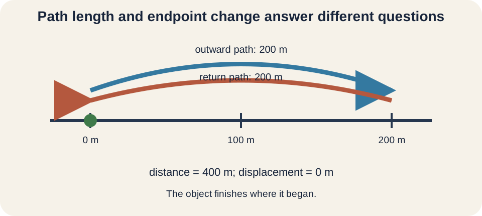
Distance is the total path length traveled and is nonnegative. In one-dimensional motion without reversal, distance equals $|\Delta x|$. With one or more reversals, distance exceeds the magnitude of displacement. In several dimensions, path shape matters even without a one-dimensional sign reversal. Keeping an endpoint arrow and a traced path separate makes the distinction visible.

Average velocity describes an interval

Average velocity is $\mathbf v_{\mathrm{avg}}=\frac{\Delta\mathbf r}{\Delta t}$ in vector notation. The numerator $\Delta\mathbf r=\mathbf r_f-\mathbf r_i$ is displacement, and the denominator $\Delta t=t_f-t_i$ is elapsed time. The horizontal fraction bar groups the complete displacement over the complete interval. In one dimension, this becomes $v_{\mathrm{avg}}=\frac{x_f-x_i}{t_f-t_i}$. Units are length per time.

Average velocity points in the direction of displacement because elapsed time is positive. It does not necessarily equal the velocity at the midpoint time. It also does not reveal reversals or pauses within the interval. Many different motion histories can share the same endpoints and time. Average quantities deliberately compress detail.

Suppose a car moves from $x_i=10.0\,\mathrm m$ at $t_i=2.0\,\mathrm s$ to $x_f=70.0\,\mathrm m$ at $t_f=7.0\,\mathrm s$. Displacement is $60.0\,\mathrm m$ and elapsed time is $5.0\,\mathrm s$. Thus $v_{\mathrm{avg}}=\frac{60.0\,\mathrm m}{5.0\,\mathrm s}=12\,\mathrm{\frac{m}{s}}$ in the positive direction. The positive sign agrees with the increase in position. The calculation says nothing about whether speed was constant between measurements.

Average speed uses total distance

Average speed is $s_{\mathrm{avg}}=\frac{d_{\mathrm{total}}}{\Delta t}$. The symbol $d_{\mathrm{total}}$ denotes total path length, not displacement. Since distance and elapsed time are nonnegative, average speed is nonnegative. It has the same units as velocity but lacks direction. Equal units do not make two quantities identical.

For a trip with no reversal along a straight line, average speed equals the magnitude of average velocity. Once the object reverses or follows a curved path, total distance can exceed displacement magnitude. Therefore $s_{\mathrm{avg}}\geq|\mathbf v_{\mathrm{avg}}|$. Equality requires the path length to equal the straight endpoint separation. This inequality is a useful reasonableness check.

A cyclist rides $120\,\mathrm m$ east in $20.0\,\mathrm s$ and returns $120\,\mathrm m$ west in $30.0\,\mathrm s$. Total time is $50.0\,\mathrm s$, displacement is zero, and distance is $240\,\mathrm m$. Average velocity is $0\,\mathrm{\frac{m}{s}}$. Average speed is $\frac{240\,\mathrm m}{50.0\,\mathrm s}=4.80\,\mathrm{\frac{m}{s}}$. The positive speed records travel that endpoint displacement omits.

Equal-distance speed averages need time weighting

Average speed is not generally the arithmetic mean of two speeds. The definition uses total distance divided by total time. Time spent at each speed provides the weighting. If equal times are spent at speeds $u$ and $v$, the arithmetic mean applies. If equal distances are traveled, a different result follows.

Suppose a traveler covers equal distance $D$ at speed $u$ and then speed $v$. Total distance is $2D$. Total time is $\frac{D}{u}+\frac{D}{v}$. Therefore $s_{\mathrm{avg}}=\frac{2D}{\frac{D}{u}+\frac{D}{v}}=\frac{2uv}{u+v}$. This is the harmonic mean of the two speeds.

Traveling equal distances at $30.0\,\mathrm{\frac{km}{h}}$ and $60.0\,\mathrm{\frac{km}{h}}$ gives $s_{\mathrm{avg}}=\frac{2(30.0)(60.0)}{30.0+60.0}=40.0\,\mathrm{\frac{km}{h}}$, not $45.0\,\mathrm{\frac{km}{h}}$. More time is spent at the slower speed. A concrete choice such as $60.0\,\mathrm{km}$ each way confirms the result. That trip takes two hours outward and one hour returning. Definition-first reasoning prevents the averaging error.

Instantaneous velocity emerges from a limit

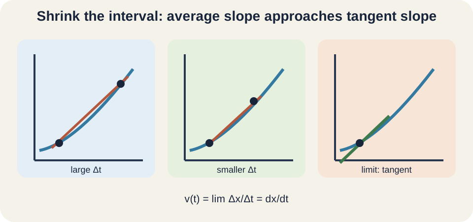
Average velocity over a shrinking interval beginning at $t$ is $\frac{\mathbf r(t+\Delta t)-\mathbf r(t)}{\Delta t}$. Let the interval approach zero. Instantaneous velocity is $\mathbf v(t)=\lim_{\Delta t\to0}\frac{\mathbf r(t+\Delta t)-\mathbf r(t)}{\Delta t}$. This limit is the derivative $\frac{d\mathbf r}{dt}$. It gives the local rate of position change.

The interval does not become an ordinary division by zero. For each nonzero $\Delta t$, a valid average ratio exists. The limit asks what value those ratios approach as the interval shrinks. If a stable limiting value exists, it defines the derivative. The instantaneous quantity is therefore built from nearby interval behavior.

In one dimension, $v(t)=\frac{dx}{dt}$. Instantaneous speed is $|v(t)|$. In several dimensions, speed is $|\mathbf v|=\sqrt{v_x^2+v_y^2+v_z^2}$. The square-root expression is the vector magnitude. Components can be negative while the magnitude remains nonnegative.

Position–time graphs encode velocity as slope

On a graph of position $x$ vertically versus time $t$ horizontally, average velocity is a secant slope. Choose two points and calculate $\frac{\Delta x}{\Delta t}$. A steeper positive secant means larger positive average velocity. A negative secant means the final position is smaller. A zero secant means equal endpoint positions, even if motion occurred between them.

Instantaneous velocity is the tangent slope at one time. A rising curve has positive velocity, a falling curve has negative velocity, and a horizontal tangent has zero velocity. Curvature tells how slope changes and therefore relates to acceleration. Position value itself does not determine velocity. An object can have negative position while moving positive.

Graph units matter. If position is in meters and time in seconds, slope is meters per second. If an axis uses kilometers and hours, slope has kilometers per hour. Convert only when the requested unit requires it. A slope without units is incomplete.

Straight and curved position graphs

A straight position–time line has constant slope and therefore constant velocity. Equal time intervals produce equal displacements. A horizontal straight line represents constant position and zero velocity. A steeper line represents greater speed magnitude. Whether it lies above or below the time axis does not determine motion direction.

A curved position–time graph has changing slope and therefore changing velocity. If the curve rises but flattens, velocity is positive while speed decreases. If it falls and becomes steeper downward, velocity is negative while speed increases. Visual steepness means slope magnitude. “Up” on a position graph is not necessarily upward physical travel.

A sharp corner represents an abrupt change in slope. The mathematical velocity may be undefined exactly at the corner because left and right tangent slopes differ. Real objects with finite forces cannot change velocity instantaneously. Such corners are idealizations or evidence that sampling missed a rapid transition. Graph smoothness carries physical meaning.

Negative velocity is not negative speed

Choose right as positive. A velocity of $-5.0\,\mathrm{\frac{m}{s}}$ means motion left at speed $5.0\,\mathrm{\frac{m}{s}}$. The negative sign communicates direction. It does not mean the object moves less than zero meters per second in magnitude. Taking absolute value gives the instantaneous speed.

Whether an object speeds up depends on velocity and acceleration signs together. If both have the same sign, speed increases in one dimension. If signs differ, speed decreases. Thus negative velocity with negative acceleration means speeding up toward the negative direction. Negative velocity with positive acceleration means slowing down while moving negative.

Language such as “backward” depends on object orientation, while positive and negative depend on coordinate choice. A car can face east while rolling west. Physics equations need the coordinate direction, not a casual label. Draw an axis arrow. Then translate verbal directions into signs.

Constant speed can accompany changing velocity

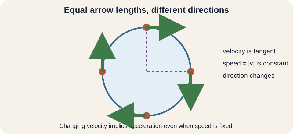
Velocity includes direction, so it can change even when magnitude remains fixed. Uniform circular motion is the clearest example. A runner moving around a circular track at constant speed continually changes velocity direction. The velocity vector is tangent to the path. Acceleration points toward the center.

After one complete lap, displacement is zero while distance equals the circumference. Average velocity over the lap is zero. Average speed equals circumference divided by lap time. Instantaneous speed remains positive throughout. These facts coexist without contradiction because they describe different aspects and intervals.

On a curved path, subtracting velocity vectors reveals direction change. Two equal-length velocity arrows at different angles have a nonzero difference. Acceleration will quantify that difference per time. Scalar speed alone cannot predict it. Vector diagrams are therefore essential for two-dimensional kinematics.

Relative velocity depends on reference frame

Velocity is measured relative to a reference frame. A passenger seated on a train has zero velocity relative to the train but nonzero velocity relative to the ground. Neither statement is inherently more correct. Each must name its frame. Displacement and velocity transform when the reference frame moves.

At ordinary speeds in Galilean mechanics, $\mathbf v_{A/C}=\mathbf v_{A/B}+\mathbf v_{B/C}$. The notation means velocity of A relative to C equals velocity of A relative to B plus velocity of B relative to C. Vectors must be added with direction. The middle reference label B cancels conceptually through the chain. A person walking forward inside a moving train has ground velocity equal to walking velocity relative to train plus train velocity relative to ground.

Suppose a train moves east at $20.0\,\mathrm{\frac{m}{s}}$ and a passenger walks west at $2.0\,\mathrm{\frac{m}{s}}$ relative to the train. Choose east positive. Ground velocity is $+20.0+(-2.0)=+18.0\,\mathrm{\frac{m}{s}}$. The passenger moves west relative to the train but east relative to the ground. Direction words require their reference object.

Measuring velocity from data

Motion sensors, video frames, GPS receivers, and timing gates estimate position at discrete times. A finite-difference estimate is $v\approx\frac{x_{i+1}-x_i}{t_{i+1}-t_i}$. This is an average velocity over a short interval. Assigning it to the interval midpoint can approximate instantaneous velocity. Smaller intervals improve time localization but can amplify position noise.

A centered difference uses data on both sides: $v(t_i)\approx\frac{x_{i+1}-x_{i-1}}{t_{i+1}-t_{i-1}}$. For smooth motion, this often estimates the tangent more accurately than a one-sided difference. It cannot be used at the first or last sample without modification. Numerical derivatives magnify measurement fluctuations. Smoothing choices must be reported because they affect results.

Uncertainty in position and time propagates into velocity. Very small time gaps can make the denominator small while position uncertainty remains comparable. Repeated trials and calibrated scales improve confidence. A graph with error bars shows whether apparent slope changes exceed measurement noise. Experimental velocity is always an estimate with resolution.

Unit conversion preserves the physical rate

Velocity units combine length and time. To convert $72.0\,\mathrm{\frac{km}{h}}$ to meters per second, multiply by conversion factors equal to one. Write $72.0\,\mathrm{\frac{km}{h}}\left(\frac{1000\,\mathrm m}{1\,\mathrm{km}}\right)\left(\frac{1\,\mathrm h}{3600\,\mathrm s}\right)=20.0\,\mathrm{\frac{m}{s}}$. Kilometers and hours cancel. The physical velocity remains the same.

Converting a vector also preserves direction. If west is negative, $-72.0\,\mathrm{\frac{km}{h}}=-20.0\,\mathrm{\frac{m}{s}}$. Conversion factors change numerical scale and unit symbols, not the sign convention. Dropping the sign during conversion loses vector information. Write direction again after the result.

Dimensional analysis catches many formula errors. Displacement divided by time can produce velocity. Distance multiplied by time cannot. A graph slope must match vertical units over horizontal units. Units are part of the reasoning, not decorative suffixes.

Common misconceptions and repairs

One misconception treats distance and displacement as synonyms. Distance follows the traveled path, while displacement connects endpoints. A round trip has positive distance and zero displacement. Therefore it has positive average speed and zero average velocity. Draw both path and endpoint arrow.

Another misconception says negative velocity means slowing down. Negative gives direction only. Speed change depends on acceleration relative to velocity. A negative velocity can become more negative and speed up. Separate sign from magnitude trend.

A third misconception takes a simple arithmetic mean of speeds without checking time. The definition is total distance divided by total time. Equal-time segments permit arithmetic averaging, while equal-distance segments produce harmonic weighting. Build totals first. The correct average follows from them.

Practice with guided feedback

First, an object moves from $x=12.0\,\mathrm m$ to $x=-8.0\,\mathrm m$ in $4.00\,\mathrm s$; find average velocity. Second, it travels $30.0\,\mathrm m$ along its path in that time; find average speed. Third, explain a negative tangent slope on an $x$–$t$ graph. Fourth, describe constant-speed circular motion using velocity. State the chosen positive direction.

Displacement is $-8.0-12.0=-20.0\,\mathrm m$, so average velocity is $\frac{-20.0\,\mathrm m}{4.00\,\mathrm s}=-5.00\,\mathrm{\frac{m}{s}}$. Average speed is $\frac{30.0\,\mathrm m}{4.00\,\mathrm s}=7.50\,\mathrm{\frac{m}{s}}$. A negative tangent slope means position decreases at that instant. In circular motion the velocity magnitude can remain constant while its tangent direction changes. Each statement distinguishes scalar magnitude from vector direction.

For a graph check, sketch a curve that rises, becomes horizontal, and then falls. Label velocity positive, zero, and negative in those regions. Make the falling curve progressively steeper and note that negative speed is not the description; speed magnitude increases. Mark one secant and one tangent. Explain their different intervals.

Retrieval and connection forward

Without looking back, define position, displacement, distance, average velocity, average speed, instantaneous velocity, and instantaneous speed. Write each rate equation with units. Explain secant and tangent slopes on a position–time graph. Give an example with zero average velocity but positive average speed. Finish by explaining how speed can remain constant while velocity changes.

Acceleration measures how velocity changes in magnitude or direction. Constant-acceleration models will integrate velocity to predict displacement. Calculus will formalize derivatives and integrals as local rate and accumulation. Momentum will multiply velocity by mass while preserving vector direction. Every later mechanics topic depends on keeping scalar speed distinct from vector velocity.

Keep one organizing statement: velocity is the rate of position change and includes direction, while speed is its nonnegative magnitude at an instant. Average velocity uses displacement, and average speed uses total distance. Position–time slope encodes velocity. Signs come from a chosen coordinate system. Graphs, vectors, units, and definitions must tell the same motion story.