Constant-Acceleration Equations

Constant acceleration makes velocity change linearly with time and position change quadratically with time. The familiar kinematic equations are consequences of those two facts rather than unrelated formulas to memorize. Each equation contains a different subset of the same five variables: displacement, initial velocity, final velocity, acceleration, and elapsed time. Selecting an equation is therefore a problem of matching known and unknown quantities. Deriving the set makes that structure visible and supplies built-in checks.

The model applies only over an interval where acceleration can reasonably be treated as constant. A car may accelerate approximately uniformly for a short interval, and an object near Earth can often use constant gravitational acceleration when air resistance is neglected. A changing thrust, substantial drag, or position-dependent force requires a different model or shorter piecewise intervals. Signs come from the chosen coordinate axis rather than from words such as “slowing.” This lesson connects definitions, graphs, algebra, units, and physical interpretation into one workflow.

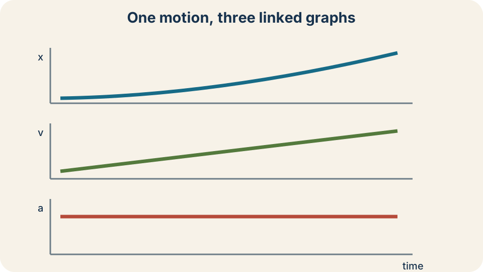
Constant acceleration appears as a horizontal line on an acceleration–time graph. Velocity is then linear because equal time intervals add equal velocity changes. Position is quadratic because the velocity itself changes linearly. Slope links each graph to the one below it. Signed area links acceleration to velocity change and velocity to displacement.

Define the five kinematic quantities

Let initial time be $t_0$ and final time be $t_f$. Elapsed time is $\Delta t=t_f-t_0$, measured in seconds. Initial position is $x_0=x(t_0)$ and final position is $x=x(t_f)$. Displacement is $\Delta x=x-x_0$, measured in metres. Displacement can be positive, negative, or zero depending on endpoints and axis.

Initial velocity is $v_0=v(t_0)$ and final velocity is $v=v(t_f)$. Velocity carries units $\frac{\mathrm{m}}{\mathrm{s}}$ and a sign indicating direction. Constant acceleration is $a=\frac{\Delta v}{\Delta t}$ with units $\frac{\mathrm{m}}{\mathrm{s}^2}$. The squared second means velocity changes by a certain number of metres per second during each second. Acceleration sign indicates the direction of velocity change, not automatically whether speed increases.

Many textbook equations set $t_0=0$ and write elapsed time simply as $t$. That convention is acceptable when stated. The variables then refer to one chosen motion interval. Values from different intervals cannot be mixed without resetting initial conditions. A diagram with labeled start and end states keeps the interval coherent.

Choose and maintain a sign convention

Select one coordinate direction as positive before assigning values. Right or upward are common choices, but either direction can be positive. Once selected, positions, displacements, velocities, and acceleration components receive signs consistently. A vector pointing opposite the positive axis has a negative component. Magnitudes such as speed remain nonnegative.

If right is positive, a car moving right has positive velocity. Braking while moving right produces acceleration to the left, so acceleration is negative. If the car later moves left while still accelerating left, both velocity and acceleration are negative and speed increases. Therefore negative acceleration does not mean slowing. Speed decreases when velocity and acceleration have opposite signs.

For vertical motion, upward-positive gives gravitational acceleration $a=-9.81\,\frac{\mathrm{m}}{\mathrm{s}^2}$ near Earth’s surface. Downward-positive gives $a=+9.81\,\frac{\mathrm{m}}{\mathrm{s}^2}$. The physical acceleration is the same in both coordinates. Equations remain consistent when every signed quantity follows one convention. Switching conventions midway creates apparent contradictions.

Derive velocity from constant acceleration

Acceleration is the time derivative of velocity: $a=\frac{dv}{dt}$. When $a$ is constant, integrate from initial time $0$ to elapsed time $t$. The left side accumulates velocity change, while the right side accumulates constant acceleration over time. The result is $v-v_0=at$. Rearranging gives $v=v_0+at$.

The same equation follows from the constant-acceleration definition $a=\frac{v-v_0}{t}$. Multiplying by time gives $at=v-v_0$. The term $at$ has units $\frac{\mathrm{m}}{\mathrm{s}^2}\cdot\mathrm{s}=\frac{\mathrm{m}}{\mathrm{s}}$. It can therefore be added to initial velocity. Units confirm the equation’s dimensional consistency.

On a velocity–time graph, the equation is a straight line. The vertical intercept is $v_0$, and the slope is $a$. Positive acceleration tilts the line upward, while negative acceleration tilts it downward. The line can cross zero velocity without acceleration changing. That crossing represents a momentary stop and possible direction reversal.

Derive displacement from velocity

Velocity is the time derivative of position: $v=\frac{dx}{dt}$. Substitute $v(t)=v_0+at$ and integrate from $0$ to $t$. The position change is $\Delta x=\int_0^t(v_0+a\tau)\,d\tau$, where $\tau$ is a dummy time variable. Integration gives $\Delta x=v_0t+\frac{1}{2}at^2$. Each term has metre units.

The term $v_0t$ is the displacement that would occur if initial velocity remained constant. The term $\frac{1}{2}at^2$ is the correction caused by velocity change. The factor one-half arises from integrating the linear term $a\tau$. It is not an arbitrary coefficient. Quadratic time dependence reflects accumulation of an already changing velocity.

Adding initial position gives $x=x_0+v_0t+\frac{1}{2}at^2$. This is a quadratic function of time when $a\ne0$. Its graph can curve upward or downward depending on acceleration sign. The derivative of this position function is $v_0+at$, which recovers velocity. Differentiating again recovers constant acceleration.

Derive displacement from average velocity

When velocity changes linearly, its average over the interval is the arithmetic mean $v_{\mathrm{avg}}=\frac{v_0+v}{2}$. This statement depends on constant acceleration. Displacement equals average velocity times elapsed time. Therefore $\Delta x=\frac{v_0+v}{2}t$. The equation contains no acceleration explicitly.

Graphically, displacement is signed area under the velocity–time line. The area of a trapezoid is average of parallel-side lengths times width. The parallel vertical sides have lengths $v_0$ and $v$, and the horizontal width is $t$. Thus trapezoid area is $\frac{v_0+v}{2}t$. Geometry and algebra give the same result.

If velocity crosses zero, signed area above and below the axis can cancel. The formula then gives displacement, not total distance traveled. Distance requires splitting at the zero crossing and adding absolute geometric areas. An average velocity of zero can accompany substantial motion. Endpoint position change and path length are different quantities.

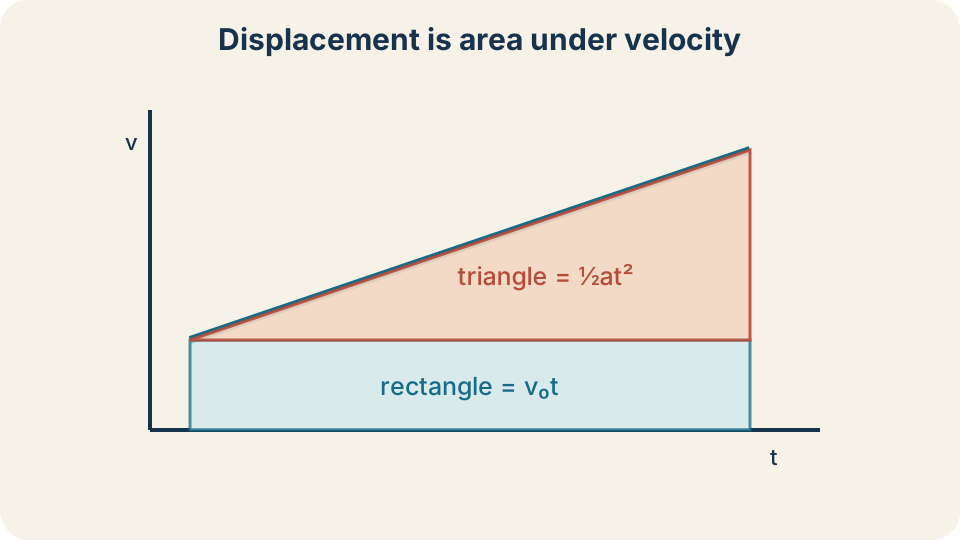
Area under a velocity–time graph is displacement. The rectangle contributes $v_0t$. The triangle contributes $\frac{1}{2}(at)t=\frac{1}{2}at^2$. Their sum gives the quadratic displacement equation. The same trapezoid area also gives average velocity times time. Signed area permits negative displacement when velocity lies below the axis.

Eliminate time to obtain the time-free equation

Sometimes elapsed time is unknown and unnecessary. Begin with $v=v_0+at$ and solve for $t=\frac{v-v_0}{a}$ when $a\ne0$. Substitute this expression into $\Delta x=\frac{v_0+v}{2}t$. The product becomes $\Delta x=\frac{v_0+v}{2}\frac{v-v_0}{a}$. The numerator uses a difference of squares.

Since $(v_0+v)(v-v_0)=v^2-v_0^2$, we get $2a\Delta x=v^2-v_0^2$. Rearranging yields $v^2=v_0^2+2a\Delta x$. Every term has units $\frac{\mathrm{m}^2}{\mathrm{s}^2}$. This equation directly connects speeds, acceleration, and displacement. It is especially useful for stopping-distance problems.

Squaring velocity removes its sign, so solving for $v$ can produce $v=\pm\sqrt{v_0^2+2a\Delta x}$. The correct branch depends on the motion stage and direction. A squared equation alone cannot determine whether the object is moving forward or backward. Other information or a time-based equation selects the sign. Do not automatically keep only the positive root when $v$ is a signed velocity.

Organize the equation set by missing variables

The equation $v=v_0+at$ omits displacement. The equation $\Delta x=v_0t+\frac{1}{2}at^2$ omits final velocity. The equation $\Delta x=vt-\frac{1}{2}at^2$ omits initial velocity and follows by substituting $v_0=v-at$. The average-velocity equation omits acceleration. The equation $v^2=v_0^2+2a\Delta x$ omits time.

Equation selection should be based on known quantities and the desired unknown. List $\Delta x$, $v_0$, $v$, $a$, and $t$ before choosing. Select an equation containing the desired variable and only one unknown overall. This approach is more reliable than matching surface wording. It also reduces unnecessary algebra.

The equations are not independent laws. They are algebraic consequences of constant acceleration and definitions. Using two equations sequentially is sometimes necessary. A result from the first becomes a known value in the second. Preserve signs and units during that transfer.

Solve a braking-distance problem

A car moves at $20.0\,\frac{\mathrm{m}}{\mathrm{s}}$ in the positive direction and brakes with constant acceleration $-5.00\,\frac{\mathrm{m}}{\mathrm{s}^2}$. At rest, final velocity is $0\,\frac{\mathrm{m}}{\mathrm{s}}$. Time is not requested, so choose $v^2=v_0^2+2a\Delta x$. Substitution gives $0=(20.0\,\frac{\mathrm{m}}{\mathrm{s}})^2+2(-5.00\,\frac{\mathrm{m}}{\mathrm{s}^2})\Delta x$. Solving yields $\Delta x=40.0\,\mathrm{m}$.

The positive displacement is physically consistent because the car continues forward while slowing. The negative acceleration does not require negative displacement. Stopping time from $v=v_0+at$ is $t=\frac{0-20.0\,\frac{\mathrm{m}}{\mathrm{s}}}{-5.00\,\frac{\mathrm{m}}{\mathrm{s}^2}}=4.00\,\mathrm{s}$. Average velocity is $10.0\,\frac{\mathrm{m}}{\mathrm{s}}$. Multiplying by $4.00\,\mathrm{s}$ independently confirms $40.0\,\mathrm{m}$.

Stopping distance scales with the square of initial speed when acceleration magnitude is fixed. Doubling $v_0$ would quadruple $v_0^2$ and therefore quadruple the braking distance. This nonlinear consequence is important for transportation safety. Reaction distance would add a separate interval before braking begins. The constant-acceleration calculation covers only the braking phase.

Solve motion starting from rest

An object starts from rest and accelerates at $3.00\,\frac{\mathrm{m}}{\mathrm{s}^2}$ for $4.00\,\mathrm{s}$. “From rest” means $v_0=0\,\frac{\mathrm{m}}{\mathrm{s}}$. Final velocity is $v=0+(3.00\,\frac{\mathrm{m}}{\mathrm{s}^2})(4.00\,\mathrm{s})=12.0\,\frac{\mathrm{m}}{\mathrm{s}}$. The positive sign matches the positive acceleration direction. Units reduce correctly to velocity.

Displacement is $\Delta x=(0)(4.00\,\mathrm{s})+\frac{1}{2}(3.00\,\frac{\mathrm{m}}{\mathrm{s}^2})(4.00\,\mathrm{s})^2=24.0\,\mathrm{m}$. Squaring time is essential. Average velocity is $\frac{0+12.0}{2}\,\frac{\mathrm{m}}{\mathrm{s}}=6.00\,\frac{\mathrm{m}}{\mathrm{s}}$. Multiplying by time gives the same $24.0\,\mathrm{m}$. Multiple routes support the result.

The final velocity is not the velocity throughout the interval. Using $12.0\,\frac{\mathrm{m}}{\mathrm{s}}$ for all four seconds would incorrectly give $48.0\,\mathrm{m}$. Velocity rises linearly from zero to twelve. Its average is six. Graph area explains the factor of one-half.

Analyze upward free fall

A ball is thrown upward at $19.6\,\frac{\mathrm{m}}{\mathrm{s}}$. Choose upward as positive and neglect air resistance. Then $v_0=+19.6\,\frac{\mathrm{m}}{\mathrm{s}}$ and $a=-9.80\,\frac{\mathrm{m}}{\mathrm{s}^2}$. At the highest point, instantaneous vertical velocity is $v=0\,\frac{\mathrm{m}}{\mathrm{s}}$. Acceleration remains downward and nonzero there.

Use $v=v_0+at$ to find $0=19.6-9.80t$ with consistent units. The time to peak is $t=2.00\,\mathrm{s}$. Height change is $\Delta y=(19.6\,\frac{\mathrm{m}}{\mathrm{s}})(2.00\,\mathrm{s})+\frac{1}{2}(-9.80\,\frac{\mathrm{m}}{\mathrm{s}^2})(2.00\,\mathrm{s})^2=19.6\,\mathrm{m}$. The positive displacement places the peak above launch point. The time value is positive and lies after launch as expected.

At the peak, zero velocity does not mean zero acceleration. The ball is momentarily at rest before reversing direction. Afterward velocity becomes negative under the same negative acceleration, so downward speed increases. The constant-acceleration equations cover ascent and descent as long as signs are maintained. Splitting at the peak can simplify questions about distance.

Solve quadratic time equations carefully

The equation $\Delta x=v_0t+\frac{1}{2}at^2$ is quadratic in time when $a\ne0$. Rearranging to standard form gives $\frac{1}{2}at^2+v_0t-\Delta x=0$. The quadratic formula may produce two time values. Each root represents an intersection of the parabolic position function with the target position. Physical interpretation determines which roots belong to the stated interval.

An upward-thrown ball can pass the same height once going up and again coming down. Both positive roots may therefore be physically meaningful. A negative root may describe the mathematical continuation before the chosen initial time. It is not automatically “wrong,” but it may lie outside the modeled experiment. State why a root is accepted or rejected.

Substitution into the original position equation checks arithmetic. Calculating velocity at each root reveals direction of travel. Units of the quadratic coefficients must be handled consistently before applying a calculator. Avoid rounding the discriminant early. The geometry of a position–time graph anticipates whether zero, one, or two real intersections should occur.

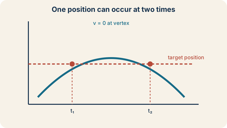
A quadratic position function can reach the same position twice. The first time may occur during upward motion and the second during downward motion. Both positive roots can be physically meaningful. A vertex represents the instant of direction reversal when velocity is zero. Root selection requires the stated time interval and motion context. Velocity at each root distinguishes the two directions.

Distinguish displacement from distance

Kinematic equations directly produce displacement, an endpoint change with sign. Distance is total path length and is nonnegative. They are equal only when motion does not reverse direction along the axis. A velocity sign change identifies a turning point. Split the interval there to compute distance.

Suppose a particle moves $5.00\,\mathrm{m}$ right and then $2.00\,\mathrm{m}$ left. Its displacement is $+3.00\,\mathrm{m}$ under right-positive convention. Its distance is $7.00\,\mathrm{m}$. A single displacement equation cannot be relabeled as distance. Motion history matters for path length.

For constant acceleration, solve $v(t)=v_0+at=0$ to locate possible reversal time. If that time lies inside the interval, calculate positions or segment displacements on each side. Add absolute segment lengths for distance. If no zero lies within the interval, velocity keeps one sign and distance equals displacement magnitude. This procedure connects algebra to path interpretation.

Interpret the graphs together

On an acceleration–time graph, constant acceleration is horizontal. Its signed area over time equals velocity change $\Delta v$. On a velocity–time graph, slope equals acceleration and signed area equals displacement. On a position–time graph, slope equals velocity and curvature reflects acceleration. The three graphs encode one motion at different derivative levels.

Positive constant acceleration makes velocity slope upward. It makes position concave up regardless of whether velocity is initially positive or negative. A negative initial velocity with positive acceleration can produce a decreasing position curve that flattens, reaches a minimum, and then rises. Concavity does not directly state motion direction. Slope supplies direction.

Graph-based reasoning checks equation results. A velocity line crossing zero predicts a position-graph vertex at the same time. Equal positive and negative velocity areas predict zero net displacement. A claimed constant acceleration should appear as a straight velocity graph. Disagreement among representations signals a sign or modeling error.

Know when the model fails

The equation set assumes one-dimensional motion and constant acceleration over the selected interval. If acceleration depends substantially on time, velocity, or position, the formulas are not exact. Air resistance often makes falling acceleration change with speed. A rocket’s acceleration may change as fuel mass and thrust vary. One constant value cannot represent the entire motion accurately.

The motion can sometimes be divided into intervals with different constant accelerations. Use the final state of one interval as the initial state of the next. Do not apply one equation across a discontinuous acceleration change without segmenting. Piecewise modeling preserves continuity of position and usually velocity. Each segment needs its own labeled conditions.

For continuously varying acceleration, calculus or numerical methods are appropriate. Integrate $a(t)$ to obtain velocity and integrate velocity to obtain position. If acceleration depends on velocity or position, solve the corresponding differential equation. The constant-acceleration equations remain useful local approximations over sufficiently short intervals. Model selection is part of the physics solution.

Follow an error-resistant workflow

First choose a positive direction and sketch the motion interval. List $\Delta x$, $v_0$, $v$, $a$, and $t$ with signs and units. Mark exactly one desired unknown. Verify that constant acceleration is a reasonable assumption. Then select an equation that contains the desired variable and known quantities.

Solve symbolically before substituting when practical. Symbolic isolation preserves structure and reduces calculator mistakes. Carry units through products and squares. If a quadratic produces multiple roots, interpret each against the interval and graph. Do not discard a negative velocity root simply because speed is nonnegative.

Finally check dimensions, signs, and magnitude. Velocity equations must produce $\frac{\mathrm{m}}{\mathrm{s}}$, displacement equations must produce metres, and squared-velocity equations must preserve $\frac{\mathrm{m}^2}{\mathrm{s}^2}$. Compare with graph slope and area. Substitute the result into an independent equation when available. A complete answer reports direction as well as magnitude.

Repair common mistakes

One mistake is selecting signs from words such as “accelerating” or “slowing.” Signs follow the coordinate axis. Compare velocity and acceleration signs to determine speed change. Another mistake is assigning gravitational acceleration as always negative. It is negative only when upward is chosen positive. If downward is positive, the gravitational component is positive instead.

Another mistake is using final velocity times total time as displacement during acceleration. The correct average is $\frac{v_0+v}{2}$ for constant acceleration. A related error omits the square on time in $\frac{1}{2}at^2$. Unit analysis exposes both problems. Metres per second times seconds gives metres, while acceleration needs seconds squared to produce metres.

A final mistake is applying the equations when acceleration changes. The formulas may still return numbers but no longer describe the stated model exactly. Another is rejecting every negative root without context. Roots, signs, and intervals carry physical information. Derivation conditions and motion diagrams decide relevance.

Retrieve and connect forward

Starting from rest at $3.00\,\frac{\mathrm{m}}{\mathrm{s}^2}$ for $4.00\,\mathrm{s}$ gives final velocity $12.0\,\frac{\mathrm{m}}{\mathrm{s}}$ and displacement $24.0\,\mathrm{m}$. An upward launch at $19.6\,\frac{\mathrm{m}}{\mathrm{s}}$ under $-9.80\,\frac{\mathrm{m}}{\mathrm{s}^2}$ reaches its peak after $2.00\,\mathrm{s}$. A $20.0\,\frac{\mathrm{m}}{\mathrm{s}}$ car braking at $-5.00\,\frac{\mathrm{m}}{\mathrm{s}^2}$ travels $40.0\,\mathrm{m}$ before stopping. Each result uses one consistent axis. Units and signs make the calculations interpretable.

The four common equations are connected derivations, not a formula bank. Linear velocity, quadratic position, trapezoid area, and time elimination express the same constant-acceleration model. Known-variable lists select efficient forms. Graphs independently predict slopes, areas, turning points, and root counts. Agreement across these representations is strong evidence of correctness.

Projectile motion applies the equations independently to perpendicular components. Horizontal acceleration may be zero while vertical acceleration is constant gravity. Work–energy methods later eliminate time through energy rather than kinematics. Calculus extends the reasoning to variable acceleration. The enduring habit is to define the model before manipulating equations.