Acceleration

Acceleration describes how velocity changes, not simply how fast an object moves. A steadily moving car can have zero acceleration. A turning car accelerates even when its speedometer reading stays constant because velocity includes direction. A slowing object accelerates opposite its velocity. These distinctions require careful vector reasoning.

The central relationship is $\mathbf a=\frac{d\mathbf v}{dt}$. Bold symbols represent vectors, $d$ signals an instantaneous change, and $t$ represents time. The SI unit is $\mathrm{\frac{m}{s^2}}$, read “metres per second per second.” It states how many metres per second velocity changes during each second. Acceleration is the rate linking velocity to time.

This lesson moves among words, diagrams, graphs, and equations. You will predict direction before calculating and attach units to numerical values. You will distinguish average acceleration over an interval from instantaneous acceleration at one moment. You will also test when constant acceleration is a justified model. The goal is reasoning rather than formula recall.

Learning goals and an opening prediction

You should define average and instantaneous acceleration in words and symbols. You should compute acceleration with units and interpret its sign. You should identify acceleration from position–time and velocity–time graphs. You should explain acceleration at constant speed. You should evaluate evidence for a constant-acceleration model.

Imagine a ball thrown straight upward after it leaves the hand. Its velocity points upward while it rises. Gravitational acceleration points downward. Opposite directions make the upward speed decrease. At the top, velocity is momentarily zero although acceleration remains downward.

Just after the ball begins falling, velocity points downward. Its acceleration still points downward. Matching directions make speed increase. Gravity did not reverse at the top. The velocity changed sign while acceleration stayed approximately constant.

Velocity must be understood first

Velocity is position change per time and includes direction. In one dimension, its sign encodes direction relative to a chosen axis. A velocity of $+5.0\,\mathrm{\frac{m}{s}}$ may mean eastward motion if east is positive. A velocity of $-5.0\,\mathrm{\frac{m}{s}}$ then means westward motion at the same speed. Speed is the magnitude $|\mathbf v|$ and does not reveal direction.

Acceleration asks how the entire velocity vector changes. A magnitude change counts as acceleration. A direction change also counts. Both can change simultaneously. Speeding, braking, and turning are therefore forms of acceleration.

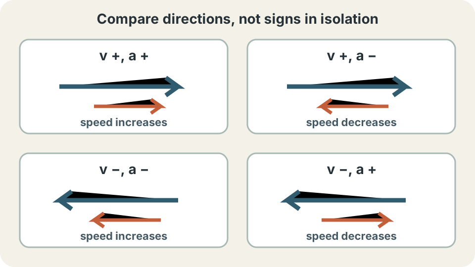
State the coordinate choice before interpreting a sign. Positive acceleration means the vector points in the positive direction. It does not automatically mean speeding up. Negative acceleration names the opposite direction rather than a motion outcome. Comparing velocity and acceleration determines the speed trend.

Average acceleration measures an interval

Average acceleration compares two velocities separated by time. Its definition is $\mathbf a_{\mathrm{avg}}=\frac{\Delta\mathbf v}{\Delta t}$. The capital Greek delta, $\Delta$, means final value minus initial value. Thus $\Delta\mathbf v=\mathbf v_f-\mathbf v_i$ and $\Delta t=t_f-t_i$. The horizontal fraction divides velocity change by elapsed time.

A runner’s eastward velocity changes from $2.0\,\mathrm{\frac{m}{s}}$ to $8.0\,\mathrm{\frac{m}{s}}$ during $3.0\,\mathrm s$. Choosing east as positive gives $\Delta v=8.0-2.0=6.0\,\mathrm{\frac{m}{s}}$. Therefore $a_{\mathrm{avg}}=\frac{6.0\,\mathrm{\frac{m}{s}}}{3.0\,\mathrm s}=2.0\,\mathrm{\frac{m}{s^2}}$. The positive result points east. Velocity increased by an average of $2.0\,\mathrm{\frac{m}{s}}$ each second.

An average does not reveal every event inside the interval. The runner might have accelerated unevenly or briefly slowed. Many velocity histories share the same endpoints. Shorter intervals provide more local information. A graph or additional measurements reveal the variations.

Units carry physical meaning

Dividing velocity by time gives $\frac{\mathrm{\frac{m}{s}}}{\mathrm s}=\mathrm{\frac{m}{s^2}}$. The squared second results from dividing by seconds twice. An acceleration of $3.0\,\mathrm{\frac{m}{s^2}}$ changes velocity by $3.0\,\mathrm{\frac{m}{s}}$ each second when constant. After one second, the change is $3.0\,\mathrm{\frac{m}{s}}$. After four seconds, it is $12.0\,\mathrm{\frac{m}{s}}$.

Dimensional reasoning exposes incorrect formulas. Multiplying acceleration by time gives velocity change. The units confirm $\left(\mathrm{\frac{m}{s^2}}\right)(\mathrm s)=\mathrm{\frac{m}{s}}$. Multiplying acceleration directly by distance does not give velocity. Units constrain algebra before numbers are substituted.

Near Earth’s surface, gravitational acceleration has magnitude $g\approx9.81\,\mathrm{\frac{m}{s^2}}$. A bare number such as “9.81” is incomplete. Other unit systems may be used if converted consistently. Every value should identify both quantity and unit. Explicit units also make scale errors easier to detect.

Instantaneous acceleration is a limiting rate

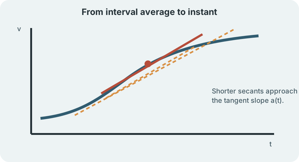
Instantaneous acceleration is approached as the averaging interval shrinks. In symbols, $\mathbf a(t)=\lim_{\Delta t\to0}\frac{\mathbf v(t+\Delta t)-\mathbf v(t)}{\Delta t}$. The limit does not divide by an interval equal to zero. It studies increasingly short nonzero intervals. Calculus calls the limiting rate $\frac{d\mathbf v}{dt}$.

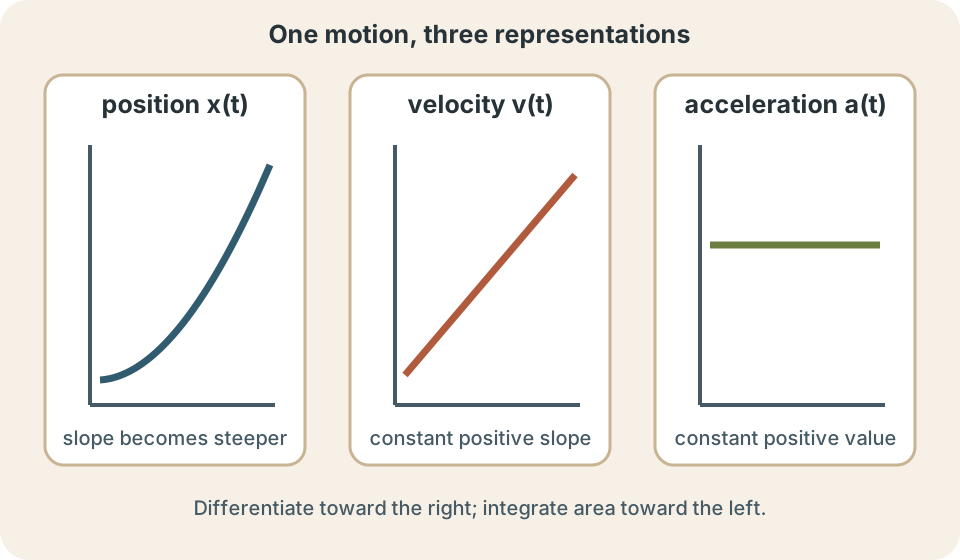
Velocity is $\mathbf v=\frac{d\mathbf r}{dt}$, so acceleration is the second derivative of position. The relationship is $\mathbf a=\frac{d^2\mathbf r}{dt^2}$. The superscript $2$ means position has been differentiated twice. It does not simply square position or time. Position, velocity, and acceleration are successive descriptions of change.

An accelerometer estimates acceleration over short sampling intervals. Short intervals improve time resolution but may amplify noise. Sensors need calibration and uncertainty estimates. A displayed value is a measurement result, not a perfect mathematical point. The derivative is the model used to interpret it.

Sign pairs determine the speed trend

In one dimension, speed increases when velocity and acceleration have the same sign. Two positive signs mean positive motion becoming more positive. Two negative signs mean negative motion becoming more negative. In both cases, $|v|$ grows. The object speeds up.

Speed decreases when velocity and acceleration have opposite signs. Positive velocity with negative acceleration approaches zero. Negative velocity with positive acceleration also approaches zero. In each case, $|v|$ shrinks. The object slows down.

Reconsider the rule if velocity crosses zero. An object can slow to rest and then speed up in the opposite direction. Velocity flips sign at the turnaround. Acceleration need not flip. Divide the description into intervals around $v=0$.

Worked example: crossing through rest

A cart’s velocity changes uniformly from $-6.0\,\mathrm{\frac{m}{s}}$ to $+2.0\,\mathrm{\frac{m}{s}}$ during $4.0\,\mathrm s$. Choose rightward as positive. The change is $\Delta v=+2.0-(-6.0)=+8.0\,\mathrm{\frac{m}{s}}$. Average acceleration is $\frac{+8.0\,\mathrm{\frac{m}{s}}}{4.0\,\mathrm s}=+2.0\,\mathrm{\frac{m}{s^2}}$. The result points rightward.

Initially, velocity is negative and acceleration is positive. Opposite signs mean the cart slows while moving left. It reaches zero velocity after $\frac{6.0\,\mathrm{\frac{m}{s}}}{2.0\,\mathrm{\frac{m}{s^2}}}=3.0\,\mathrm s$. The compound units reduce to seconds. The cart reverses at that instant.

During the final $1.0\,\mathrm s$, both signs are positive. The cart speeds up while moving right. Its velocity increases to $+2.0\,\mathrm{\frac{m}{s}}$. Calling the entire interval only “speeding up” would be wrong. A timeline split at the turnaround gives the full story.

Velocity–time graphs reveal acceleration

On a velocity–time graph, average acceleration is secant slope. Slope is vertical change divided by horizontal change. Therefore $a_{\mathrm{avg}}=\frac{\Delta v}{\Delta t}$. A horizontal segment has zero acceleration. Rising and falling lines have positive and negative acceleration, respectively.

Instantaneous acceleration is tangent slope. A curved velocity graph represents changing acceleration. Steeper tangent slopes have greater acceleration magnitude. A horizontal tangent gives zero instantaneous acceleration. Its graph height can still represent nonzero velocity.

Area under a velocity–time graph represents displacement. Its units are $\left(\mathrm{\frac{m}{s}}\right)(\mathrm s)=\mathrm m$. Area under an acceleration–time graph represents velocity change. Its units are $\left(\mathrm{\frac{m}{s^2}}\right)(\mathrm s)=\mathrm{\frac{m}{s}}$. Axes and units identify which interpretation applies.

Position–time graphs reveal acceleration indirectly

Position–time slope is velocity. A straight position graph has constant velocity and zero acceleration. A slope growing more positive indicates positive acceleration. A slope becoming more negative indicates negative acceleration. Acceleration tells how the position slope changes.

Concavity provides a shortcut. A concave-up position graph has increasing slope and positive acceleration. A concave-down graph has decreasing slope and negative acceleration. Whether the graph rises or falls is a separate question. A decreasing concave-up graph shows negative velocity with positive acceleration.

Graph height is not acceleration. A high position only locates the object relative to the origin. A position turning point has zero velocity because its slope is zero. Acceleration there depends on concavity. Separating value, slope, and slope change prevents common errors.

Constant speed can include acceleration

Velocity is a vector, so changing its direction creates acceleration. In uniform circular motion, velocity is tangent to the path. A moment later, that tangent points elsewhere. The vector difference points approximately toward the center. The limiting acceleration is called centripetal acceleration.

Its magnitude is $a_c=\frac{v^2}{r}$, where $v$ is speed and $r$ is radius. The fraction divides squared speed by radius. Units become $\frac{\mathrm{\frac{m^2}{s^2}}}{\mathrm m}=\mathrm{\frac{m}{s^2}}$. Greater speed greatly raises acceleration because it is squared. A larger radius lowers acceleration at the same speed.

Centripetal acceleration is perpendicular to velocity in ideal uniform circular motion. It changes direction without changing speed. A real vehicle may also have tangential acceleration. Then speed and direction change together. Vector components combine the radial and tangential effects.

Components organize multidimensional acceleration

In two dimensions, write $\mathbf a=a_x\hat{\mathbf i}+a_y\hat{\mathbf j}$. Unit vectors $\hat{\mathbf i}$ and $\hat{\mathbf j}$ point along positive coordinate axes. Components $a_x$ and $a_y$ have signs and acceleration units. Each is a velocity-component derivative. Thus $a_x=\frac{dv_x}{dt}$ and $a_y=\frac{dv_y}{dt}$.

Projectile motion often assumes $a_x=0$ and $a_y=-g$ when upward is positive. Horizontal velocity then remains constant. Vertical velocity changes by about $-9.81\,\mathrm{\frac{m}{s}}$ each second. Overall velocity changes in magnitude and direction. Components keep perpendicular changes separate.

Acceleration magnitude is $|\mathbf a|=\sqrt{a_x^2+a_y^2}$ for perpendicular Cartesian components. The square root follows from the Pythagorean theorem. An angle describes direction, but component signs determine the quadrant. Units accompany each component and magnitude. An inverse tangent alone can select the wrong quadrant.

Constant acceleration is a model

Constant acceleration means the acceleration vector does not change during the chosen interval. Velocity then follows $\mathbf v=\mathbf v_0+\mathbf a\Delta t$. The subscript zero marks the initial velocity. Position changes quadratically because velocity changes linearly. These equations follow from the assumption rather than defining acceleration.

A nearly straight velocity–time graph supports approximate constant acceleration. Equal velocity changes over equal time intervals provide similar evidence. Experimental scatter prevents perfect equality. Residuals and uncertainty help judge deviations. The model may work briefly and fail over longer intervals.

Air drag, changing engine force, and varying slope can change acceleration. Gravity also varies with location, although a constant value often works near Earth’s surface. State the approximation and its domain. Do not choose constant-acceleration equations merely because acceleration appears. First justify the model from assumptions or data.

Measurement and uncertainty

Acceleration can be estimated by differentiating measured velocity. Differentiation subtracts nearby data and divides by short time. It therefore magnifies random variation. Smoothing can reveal trends but can erase real rapid changes. The analysis method should be reported.

Suppose velocities are $3.2\pm0.1\,\mathrm{\frac{m}{s}}$ and $5.8\pm0.1\,\mathrm{\frac{m}{s}}$ separated by $1.00\pm0.01\,\mathrm s$. The central estimate is $\frac{5.8-3.2}{1.00}=2.6\,\mathrm{\frac{m}{s^2}}$. Extra calculator digits do not improve the data. Uncertainty propagation should include both velocities and elapsed time. Reporting $2.600000\,\mathrm{\frac{m}{s^2}}$ would imply false precision.

Sensor alignment also matters. A tilted accelerometer mixes gravitational and translational components. Video tracking can suffer scale and perspective error. Repeated trials reveal variability but not every bias. A defensible result reports units, uncertainty, method, and limitations.

Common misconceptions and repairs

Negative acceleration does not always mean slowing down. Negative means the vector points along the negative axis. Negative velocity with negative acceleration produces increasing speed. Draw arrows or use a sign table. Replace the slogan with “opposite signs mean slowing in one dimension.” This repaired statement remains valid until the velocity changes sign.

Zero velocity does not imply zero acceleration. A thrown ball at its highest point is an example. Its velocity is momentarily zero while gravity still accelerates it downward. Conversely, constant nonzero velocity means zero acceleration. Value and rate of change are different properties.

Constant speed does not always imply zero acceleration. Circular motion changes velocity direction continuously. Graph height also should not be confused with slope. On a velocity graph, height is velocity and slope is acceleration. Naming axes and units repairs both mistakes.

Problem-solving routine

Define the system, coordinate axis, and positive direction. List known velocities and times with units. Predict acceleration direction before calculating. Select an interval, derivative, graph slope, or component model. Write the symbolic relationship before inserting values.

Compute $\Delta v=v_f-v_i$ in that order. Divide by the positive elapsed time and retain units. Interpret the sign as direction. Compare it with velocity to interpret speed. Split the narrative if velocity crosses zero.

Translate the result into a sentence. For example, $-2.5\,\mathrm{\frac{m}{s^2}}$ means velocity changes by $-2.5\,\mathrm{\frac{m}{s}}$ per second over the interval. Check graph slope, units, and signs independently. State assumptions such as constant acceleration. A number becomes an explanation only when its physical meaning is explicit.

Practice and connection forward

A cyclist’s eastward velocity changes from $+4.0\,\mathrm{\frac{m}{s}}$ to $+10.0\,\mathrm{\frac{m}{s}}$ in $3.0\,\mathrm s$. The velocity change is $+6.0\,\mathrm{\frac{m}{s}}$. Average acceleration is $+2.0\,\mathrm{\frac{m}{s^2}}$. Matching positive signs mean speeding up. The acceleration points east.

A cart moves left at $-7.0\,\mathrm{\frac{m}{s}}$ with acceleration $+1.4\,\mathrm{\frac{m}{s^2}}$ for $5.0\,\mathrm s$. Its velocity change is $(+1.4)(5.0)=+7.0\,\mathrm{\frac{m}{s}}$. Final velocity is zero. The cart slows to rest without yet reversing. Multiplication units reduce to $\mathrm{\frac{m}{s}}$.

Without looking back, define both forms of acceleration and explain $\mathrm{\frac{m}{s^2}}$. Sketch a velocity graph with positive acceleration. Sketch a position graph with negative velocity but positive acceleration. Explain why a turning car accelerates at constant speed. The next lessons derive motion equations and connect net force to acceleration.