Projectile Motion

Projectile motion is two-dimensional motion under gravity after an object loses contact with its launcher. In the ideal model, gravity is the only force during flight. Horizontal and vertical components follow separate equations because gravity points vertically. They remain linked by one shared time variable. This component structure turns a curved path into two familiar one-dimensional motions.

The horizontal component has constant velocity when air resistance is neglected. The vertical component has constant downward acceleration. Their combination produces a parabolic trajectory in a flat, uniform gravitational field. The object’s velocity changes continuously even when its speed may momentarily reach a minimum. At the highest point, vertical velocity is zero but horizontal velocity generally remains.

This lesson builds the model from a free-body diagram and vector components. It treats horizontal launches, angled launches, unequal launch and landing heights, and trajectory equations. Every numerical example includes units and a sign convention. Energy and symmetry provide independent checks. The final section identifies when drag, curvature, or changing gravity invalidates the simple model.

Learning objectives and an opening prediction

After this lesson, you should state the assumptions of ideal projectile motion. You should resolve initial velocity into horizontal and vertical components. You should write position and velocity equations for both directions. You should use one component to determine time and the other to determine a requested distance or velocity. You should evaluate whether a result fits the physical model.

Imagine dropping one ball while launching another horizontally from the same height at the same instant. In the ideal model, both have identical initial vertical velocity and identical vertical acceleration. They therefore reach the ground at the same time. The launched ball travels horizontally while it falls. Horizontal motion does not delay vertical fall.

Now launch an object upward at an angle. Its upward velocity decreases because acceleration points downward. At the top, the vertical component becomes zero for an instant. Gravity remains nonzero and immediately makes the vertical component downward. The projectile does not “hang” without acceleration.

Define the ideal projectile model

Treat the projectile as a particle after release. Neglect air resistance, lift, spin forces, and propulsion. Approximate gravitational acceleration as uniform with magnitude $g=9.81\,\mathrm{\frac{m}{s^2}}$ near Earth’s surface. Use a flat Cartesian coordinate system over a distance small compared with Earth’s radius. Choose upward as positive $y$.

The free-body diagram contains only weight $\mathbf F_g=m\mathbf g$. Newton’s second law gives $m\mathbf a=m\mathbf g$. Mass cancels, leaving $\mathbf a=\mathbf g$. This explains why ideal projectiles of different mass share the same acceleration. It does not claim drag affects all objects equally.

With positive $x$ horizontal and positive $y$ upward, acceleration components are $a_x=0$ and $a_y=-g$. The negative sign records direction. If a different coordinate convention is chosen, signs change consistently. The physics does not depend on the naming of positive axes. Write the convention before equations.

Resolve the initial velocity vector

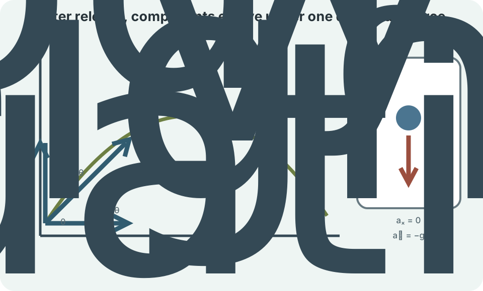
Let launch speed be $v_0$ at angle $\theta$ above the horizontal. The horizontal component is $v_{0x}=v_0\cos\theta$. The vertical component is $v_{0y}=v_0\sin\theta$. The subscript zero marks initial values. The $x$ and $y$ subscripts identify directions.

These equations follow from a right triangle whose hypotenuse is $\mathbf v_0$. Cosine relates the adjacent horizontal side to the hypotenuse. Sine relates the opposite vertical side. The angle must be measured from the horizontal for these assignments. An angle measured from vertical would swap the roles.

If $v_0=20.0\,\mathrm{\frac{m}{s}}$ and $\theta=30.0^\circ$, then $v_{0x}=17.3\,\mathrm{\frac{m}{s}}$ and $v_{0y}=10.0\,\mathrm{\frac{m}{s}}$. Components retain velocity units. Their squared sum returns $v_0^2$ within rounding. This Pythagorean check detects swapped or mistyped components. Both component signs are positive for a launch upward and to the right.

Write horizontal and vertical equations

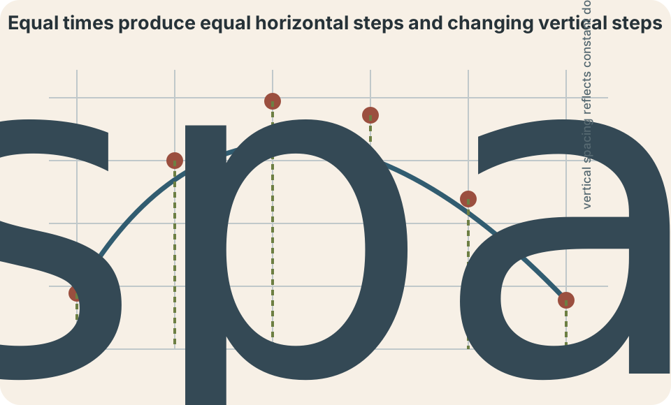
Horizontal acceleration is zero, so horizontal velocity remains $v_x(t)=v_{0x}$. Horizontal position is $x(t)=x_0+v_{0x}t$. The symbol $x_0$ is initial horizontal position. The relation assumes the chosen ground frame is inertial enough for the problem. Time $t$ is measured from launch.

Vertical velocity is $v_y(t)=v_{0y}-gt$. Vertical position is $y(t)=y_0+v_{0y}t-\frac{1}{2}gt^2$. The symbol $y_0$ is initial height. Both follow constant-acceleration kinematics. The same $t$ appears in horizontal and vertical equations.

Do not create separate horizontal and vertical times. There is one physical flight and one clock. Often the vertical equation determines flight time because landing height is known. That time is then substituted into the horizontal equation. The components are dynamically independent but temporally synchronized.

Position and velocity vectors evolve differently

The position vector is $\mathbf r(t)=x(t)\hat{\mathbf i}+y(t)\hat{\mathbf j}$. Unit vector $\hat{\mathbf i}$ points along positive $x$, and $\hat{\mathbf j}$ points along positive $y$. Velocity is $\mathbf v(t)=v_x(t)\hat{\mathbf i}+v_y(t)\hat{\mathbf j}$. Acceleration is $\mathbf a=-g\hat{\mathbf j}$. Vector notation packages both component equations.

Horizontal velocity remains constant in the ideal model. Vertical velocity changes linearly with time. The speed is $v=\sqrt{v_x^2+v_y^2}$. Speed is scalar magnitude and cannot be negative. Velocity direction satisfies $\tan\phi=\frac{v_y}{v_x}$ when quadrants are handled correctly.

At the highest point, $v_y=0$ but $v_x=v_{0x}$. Unless the launch is purely vertical, total speed is not zero. Acceleration is still $-g\hat{\mathbf j}$. Position can be momentarily extremal in one direction while motion continues in another. Component thinking prevents the “stops at the top” misconception.

Derive the parabolic trajectory

Start with $x=x_0+v_0\cos\theta\,t$. Solve for time to obtain $t=\frac{x-x_0}{v_0\cos\theta}$. This requires a nonzero horizontal component. The expression says horizontal displacement divided by constant horizontal velocity equals elapsed time. Substitute it into the vertical position equation to eliminate time.

The resulting trajectory is $y=y_0+(x-x_0)\tan\theta-\frac{g(x-x_0)^2}{2v_0^2\cos^2\theta}$. The first term fixes initial height. The linear term records the initial launch slope. The quadratic term records downward curvature from gravity. The squared horizontal displacement makes this a quadratic function of $x$.

The coefficient of $(x-x_0)^2$ is negative for ordinary positive $g$, so the parabola opens downward. The linear term contains the launch slope $\tan\theta$. At $x=x_0$, the equation returns $y=y_0$. Air resistance generally destroys the exact parabolic form. A measured nonparabolic path can therefore reveal model limitations.

Worked example: horizontal launch

A ball leaves a table horizontally at $v_{0x}=6.00\,\mathrm{\frac{m}{s}}$ from height $h=1.25\,\mathrm m$. Set launch point $y_0=1.25\,\mathrm m$ and ground $y=0$. Initial vertical velocity is zero. The vertical equation is $0=1.25\,\mathrm m-\frac{1}{2}(9.81\,\mathrm{\frac{m}{s^2}})t^2$. Solve for the positive time.

Rearranging gives $t=\sqrt{\frac{2(1.25\,\mathrm m)}{9.81\,\mathrm{\frac{m}{s^2}}}}=0.505\,\mathrm s$. Metres cancel, leaving seconds squared inside the square root. Taking the square root produces seconds. The positive root describes time after launch. The negative root is excluded because it refers to an earlier mathematical time.

Horizontal range is $\Delta x=v_{0x}t=(6.00\,\mathrm{\frac{m}{s}})(0.505\,\mathrm s)=3.03\,\mathrm m$. Vertical impact velocity is $v_y=-gt=-4.95\,\mathrm{\frac{m}{s}}$. Horizontal velocity remains $+6.00\,\mathrm{\frac{m}{s}}$. Impact speed is $\sqrt{(6.00)^2+(4.95)^2}\,\mathrm{\frac{m}{s}}=7.78\,\mathrm{\frac{m}{s}}$. Direction is below the positive horizontal.

Same-height angled launch

Suppose launch and landing heights are equal. Set vertical displacement to zero as $0=v_0\sin\theta\,t-\frac{1}{2}gt^2$. Factor $t$ to obtain one root $t=0$ at launch. The nonzero root is $T=\frac{2v_0\sin\theta}{g}$. The symbol $T$ is total flight time.

Substitute $T$ into horizontal displacement. Range is $R=v_0\cos\theta\,T=\frac{v_0^2\sin(2\theta)}{g}$. The double-angle identity $2\sin\theta\cos\theta=\sin(2\theta)$ produces the final form. Horizontal speed determines how quickly distance accumulates. Vertical speed determines how long accumulation lasts.

The same-height range formula applies only to the ideal model. It assumes equal launch and landing elevations. It also assumes no drag and constant $g$. A nonzero horizontal component is implicit in its ordinary trajectory interpretation. Specialized formulas should always be tied to their assumptions.

Maximum height above launch follows from $v_y^2=v_{0y}^2-2g\Delta y$. At the top, $v_y=0$, so $H=\frac{v_0^2\sin^2\theta}{2g}$. This $H$ is rise above launch, not necessarily height above ground. Flight time upward is $\frac{v_0\sin\theta}{g}$. Equal-height motion is symmetric in time.

Worked example: angled launch

Launch a projectile at $v_0=24.0\,\mathrm{\frac{m}{s}}$ and $\theta=40.0^\circ$, landing at launch height. Components are $v_{0x}=18.4\,\mathrm{\frac{m}{s}}$ and $v_{0y}=15.4\,\mathrm{\frac{m}{s}}$. The flight time is $T=\frac{2(15.4\,\mathrm{\frac{m}{s}})}{9.81\,\mathrm{\frac{m}{s^2}}}=3.15\,\mathrm s$. Units reduce to seconds. The calculation assumes a level landing surface.

Range is $R=(18.4\,\mathrm{\frac{m}{s}})(3.15\,\mathrm s)=58.0\,\mathrm m$. Equivalently, use $\frac{v_0^2\sin(80.0^\circ)}{g}$. Agreement between methods is a check. Rounding components too early can cause small disagreement. Keep guard digits until the final result.

Maximum rise is $H=\frac{(15.4\,\mathrm{\frac{m}{s}})^2}{2(9.81\,\mathrm{\frac{m}{s^2}})}=12.1\,\mathrm m$. At the top, velocity is horizontal with magnitude $18.4\,\mathrm{\frac{m}{s}}$. On return to launch height, ideal speed again equals $24.0\,\mathrm{\frac{m}{s}}$. Its vertical component has reversed sign. Energy conservation provides that final check.

Complementary launch angles and range

For equal-height ideal motion, range depends on $\sin(2\theta)$. Angles $\theta$ and $90^\circ-\theta$ have the same sine of twice the angle. They therefore produce equal ranges at equal speed. A low-angle trajectory is flatter and shorter in time. A high-angle trajectory rises higher and remains aloft longer.

The maximum of $\sin(2\theta)$ is one. This occurs when $2\theta=90^\circ$, so $\theta=45^\circ$. Thus $45^\circ$ maximizes ideal same-height range for a fixed speed. This conclusion changes when launch and landing heights differ. Air drag can also shift the optimal angle below $45^\circ$.

Equal range does not mean equal trajectory. Complementary angles have different flight times, maximum heights, and impact directions. A practical launcher may face obstacles or time constraints. Range is only one design criterion. State what quantity is being optimized.

Unequal launch and landing heights

When final height differs from initial height, do not use the same-height time or range formulas. Write $\Delta y=v_{0y}t-\frac{1}{2}gt^2$ with the actual signed displacement. Rearrange into a quadratic equation in $t$. Solve and select physically relevant roots. Then use horizontal motion.

A projectile launched from a cliff may have one positive time root and one negative root. The negative root represents where the mathematical parabola would have crossed the landing height before launch. It is not part of the modeled flight interval. In other geometries, two positive roots can represent crossing the same height on the way up and down. Context selects the event.

Keep $y_0$ and $y_f$ explicit when signs feel uncertain. Write $y_f=y_0+v_{0y}t-\frac{1}{2}gt^2$. Substituting actual coordinate values is safer than memorizing “drop height” signs. Sketch the coordinate axis beside the path. Geometry should predict whether vertical displacement is positive or negative.

Energy provides an independent speed check

With gravity as the only force, mechanical energy is conserved. The relation is $\frac{1}{2}mv^2+mgy=\text{constant}$. The symbol $m$ is projectile mass, $v$ is speed, $g$ is gravitational acceleration magnitude, and $y$ is vertical coordinate. Mass cancels when comparing two positions. Speed depends on height change rather than path shape.

Between launch and another point, $v^2=v_0^2+2g(y_0-y)$. The height difference appears with a sign that increases speed below launch. If the projectile lands below launch, final speed exceeds initial speed. If it returns to launch height, speeds match. This equation gives magnitude but not direction.

Component kinematics supplies direction. Energy cannot determine horizontal versus vertical velocity by itself. Combining energy with constant $v_x$ can recover $|v_y|$. The sign of $v_y$ follows whether the projectile is rising or falling. Independent methods strengthen verification.

Mass independence and air resistance

Mass cancels from $m\mathbf a=m\mathbf g$ when gravity is the only force. Two ideal projectiles with the same initial position and velocity follow the same trajectory regardless of mass. This is gravitational equivalence in the simplified local model. Shape and density do not appear. The conclusion is conditional.

With drag, force can depend on speed, area, shape, and fluid density. A common quadratic model is $\mathbf F_D=-\frac{1}{2}C_D\rho_{\mathrm{air}}A v^2\hat{\mathbf v}$. The coefficient $C_D$ is dimensionless drag coefficient, $A$ is reference area, and $\hat{\mathbf v}$ is velocity direction. Dividing by mass gives a mass-dependent acceleration contribution. Ideal mass independence can then fail.

Drag reduces range and breaks horizontal velocity constancy. The descending path is usually steeper than the ascending path. The optimal range angle changes. Closed-form elementary equations may no longer exist. Numerical integration becomes useful.

Relative motion and moving launchers

Launch velocity depends on the reference frame. If a person on a moving cart throws a ball, ground-frame velocity is the vector sum of throw velocity relative to the cart and cart velocity relative to ground under Galilean conditions. Components must be transformed before using projectile equations. The gravitational acceleration is approximately the same in these ordinary frames. State the frame for every velocity.

A package released from an airplane retains the airplane’s horizontal velocity at release. It does not drop straight down in the ground frame. In the airplane’s constant-velocity frame, it can appear to fall below the release point. Both descriptions are consistent. Different frames assign different horizontal positions.

Wind and air motion matter only when drag is included. Drag depends on projectile velocity relative to air, not automatically relative to ground. A tailwind changes that relative velocity. The ideal no-drag model ignores wind completely. Model additions must use the correct relative quantity.

Experimental graphs reveal component structure

A motion-tracking video can provide $x(t)$ and $y(t)$. Ideal horizontal position plotted against time is linear. Its slope is $v_{0x}$. Ideal vertical position is quadratic. A fitted second-order coefficient should correspond to $-\frac{1}{2}g$ under upward-positive convention.

Horizontal velocity versus time should be constant. Vertical velocity versus time should be linear with slope $-g$. Scatter arises from pixel resolution, frame timing, calibration, and point tracking. Systematic curvature in $x(t)$ can indicate drag or camera perspective. Residuals test the model.

Units must be calibrated from image distance and frame rate. Pixels are not metres until a scale is established. Frame number is not seconds until divided by frames per second. Perspective can make one scale inappropriate across depth. Measurement geometry matters as much as algebra.

Common mistakes and repairs

One mistake is assigning acceleration zero at the highest point. Only vertical velocity is zero there. Gravitational acceleration remains $-9.81\,\mathrm{\frac{m}{s^2}}$. Draw the free-body diagram at the top. The force has not disappeared.

Another mistake is using total launch speed in the horizontal equation. Resolve $v_0$ first. Horizontal motion uses $v_0\cos\theta$, while vertical motion uses $v_0\sin\theta$. Verify that component squares recover $v_0^2$. Angles are not interchangeable.

A third mistake is using the same-height range formula for a cliff launch. Return to component equations. Solve the actual vertical displacement for time. Use that time horizontally. Specialized formulas should never override geometry.

A reliable projectile workflow

First draw the path, coordinate axes, and free-body diagram. State ideal assumptions and the reference frame. Record initial and final coordinates. Resolve the initial velocity. Attach units to every known quantity.

Second write one horizontal and one vertical equation with the same $t$. Choose the component containing enough information to solve for time or another unknown. Reject roots outside the physical interval. Substitute the shared time into the other component. Keep signs tied to the chosen axes.

Third verify the result. Check units and limiting cases. Use energy for speed when only gravity acts. Test whether horizontal velocity remains constant and whether vertical acceleration has the correct sign. Explain how drag or unequal heights would change the conclusion.

Retrieval practice and synthesis

Without looking back, write the four core component equations for $x(t)$, $y(t)$, $v_x(t)$, and $v_y(t)$. Define every symbol and sign. Explain why one time variable appears in all four. State the assumptions that make $a_x=0$. Describe the velocity at the highest point.

Rework the horizontal-launch example with height $5.00\,\mathrm m$ and horizontal speed $10.0\,\mathrm{\frac{m}{s}}$. Determine time, range, vertical impact velocity, and impact speed. Carry units through every line. Use energy to verify the speed. State why projectile mass is unnecessary.

Compare $30^\circ$ and $60^\circ$ launches at equal speed and equal landing height. Explain why their ideal ranges match. Compare their flight times and maximum heights. Identify which mathematical factor creates equal range. State two real effects that can break the comparison.