Free-Body Diagrams

A free-body diagram is an interaction inventory for one chosen system. It replaces visual scene clutter with external force vectors that can be added mathematically. Its value is not artistic realism. A disciplined diagram prevents omitted forces, invented forces, double counting, and mixing forces that act on different objects. This lesson develops a repeatable construction method and then connects each arrow to Newton’s component equations.

Choose exactly one system first

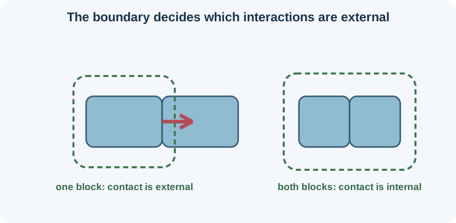
The system is the object or collection of objects whose motion will be analyzed. Draw or name its boundary before listing forces. An interaction crossing that boundary is external. An interaction between parts inside the boundary is internal. Newton’s second-law force sum contains external forces on the selected system.

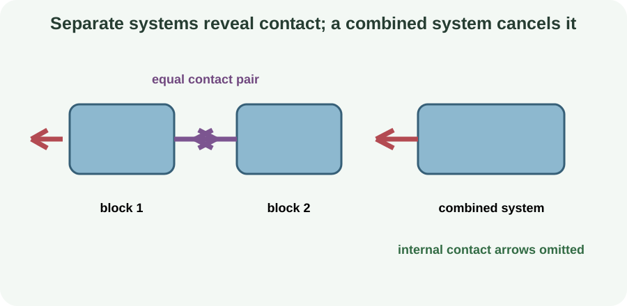
A block can be one system. Two touching blocks can instead be treated together as one larger system. The best choice depends on the desired unknown. A combined system often removes internal contact forces from the equation. Separate systems reveal those contact forces when they are needed.

Changing the boundary changes the diagram but not the physical event. A rope tension may be external to a hanging mass and internal to a mass-rope system. Both choices can be valid when consistently modeled. State the system near every free-body diagram. Without that label, force arrows have ambiguous ownership.

Replace the system with a simple representation

Represent the selected system by a point, box, or simple outline. The shape does not need to resemble the object. The purpose is to provide a common origin or attachment location for force arrows. For a particle model, all arrows may begin at one point. For torque problems, application points may later matter.

Remove surrounding objects from the free-body diagram. Their effects remain through force arrows. A table becomes an upward normal-force arrow on a book. Earth becomes a downward gravitational-force arrow. A rope becomes a tension arrow along the rope direction.

Do not redraw the entire scene and call it a free-body diagram. A scene diagram can show geometry, motion, and multiple objects. A free-body diagram isolates one system and only its external interactions. Keeping both drawings separate can be helpful. Their purposes are complementary rather than interchangeable.

Inventory interactions by asking for agents

For every force, identify an external agent acting on the system. Ask what touches the system. Then ask what acts at a distance. Contact agents include surfaces, ropes, springs, fluids, and people. Long-range agents include Earth and electrically or magnetically interacting objects.

Label each force by both type and agent when ambiguity is possible. For example, $\mathbf F_{\text{table on book}}$ identifies who acts on whom. Shorter notation such as $\mathbf F_N$ is convenient after the interaction is clear. A label like “applied force” is incomplete if several agents push. Agent-based naming prevents forces from appearing without a physical source.

Every real force corresponds to an interaction. Velocity is not an interaction. Acceleration is not an interaction. The product $m\mathbf a$ is the result of the net force, not an additional force arrow. If an arrow has no external agent, question whether it belongs.

Draw force vectors with meaningful directions

An arrow points in the direction of the force on the system. Its length may represent magnitude when the diagram is drawn approximately to scale. Place the tail on the system representation. Label the arrow clearly. Avoid using identical labels for distinct forces.

Do not choose arrow directions merely to make an equation balance. Direction comes from interaction physics. Gravity points toward the attracting body. A taut rope pulls away from the object along the rope. A surface normal pushes perpendicular to contact. Friction lies along contact and opposes relative slipping or impending slipping.

An unknown force direction can be assigned as a coordinate assumption when physics does not fix it. A negative solved component then indicates the actual direction is opposite the assumption. This algebraic convention differs from drawing a known force incorrectly. State assumed directions. Let signs communicate the result.

Recognize gravitational force

Near Earth’s surface, gravitational force is $\mathbf F_g=m\mathbf g$. Its magnitude is $mg$, and its direction is downward toward Earth’s center. Mass $m$ is measured in kilograms. Gravitational acceleration magnitude $g$ is approximately $9.80\,\mathrm{m\,s^{-2}}$. The resulting force unit is the newton, $1\,\mathrm N=1\,\mathrm{kg\,m\,s^{-2}}$.

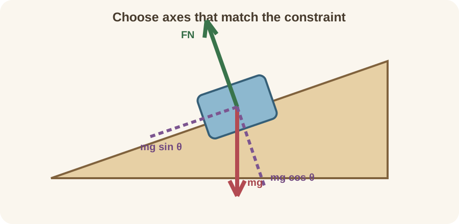
For a $5.00\,\mathrm{kg}$ block, weight magnitude is $(5.00\,\mathrm{kg})(9.80\,\mathrm{m\,s^{-2}})=49.0\,\mathrm N$. The arrow points vertically downward even when the block sits on an incline. Tilting the surface does not tilt gravity. Coordinate components may align partly along the incline, but the physical vector remains downward. Checking the arrow against Earth’s location verifies its direction.

Weight and mass are different quantities. Mass measures inertia and uses kilograms. Weight is a force and uses newtons. A free-body diagram contains the weight force arrow, not a mass arrow. Units make this distinction visible.

Recognize the normal force

A normal force is a contact force perpendicular to a surface. The word normal means perpendicular in this context. Its direction follows contact geometry. A horizontal table pushes vertically on a resting book. An incline pushes perpendicular to the incline.

Normal force is not automatically equal to $mg$. It equals weight magnitude only in a particular horizontal equilibrium with no other vertical forces. An additional downward push increases it. An upward pull can reduce it. On an incline, it balances only the perpendicular component of other forces when perpendicular acceleration is zero.

A surface can push but not pull in an ordinary contact model. If equations require a negative normal force, contact may have ended or the assumed configuration may be impossible. This physical constraint provides a reasonableness check. Solving the component equation determines the magnitude. Memorizing $F_N=mg$ bypasses the actual mechanics.

Recognize tension and spring forces

Ideal tension acts along a taut rope, cable, or string. A rope pulls an attached object away from the object and along the rope. It does not push in the ideal flexible model. For a massless rope over an ideal pulley, tension magnitude may be uniform. Real ropes and pulleys can violate that simplification.

Draw one tension arrow for each rope segment directly pulling the chosen system. Two segments can produce two tension forces. Equal labels require a justified ideal-rope model. A knot, pulley, or massive rope may need its own free-body diagram. Geometry determines the direction of each tension.

An ideal spring exerts $\mathbf F_s=-k\mathbf x$ along its deformation direction. The constant $k$ has units $\mathrm{N\,m^{-1}}$. The negative sign indicates a restoring force opposite displacement from equilibrium. A compressed spring pushes, while a stretched spring pulls. The spring itself is the external agent when it lies outside the selected system.

Determine friction direction from relative motion

Friction acts parallel to the contact surface. Kinetic friction opposes actual relative sliding. Static friction opposes the relative sliding that would otherwise occur. It does not automatically point opposite the object’s velocity. A rolling wheel can require static friction in a direction that surprises a motion-based guess.

The kinetic-friction magnitude is often modeled as $f_k=\mu_kF_N$. The coefficient $\mu_k$ is dimensionless. The static-friction condition is $0\leq f_s\leq\mu_sF_N$. Static friction adjusts up to a maximum rather than always equaling it. Solve for required static friction before comparing with the limit.

To choose direction, imagine the contact without friction. Determine which way the surfaces would slide relative to each other. Static friction opposes that tendency. For kinetic friction, use known relative sliding. This counterfactual method is more reliable than a memorized “friction points backward” rule.

Keep motion arrows off the force inventory

Velocity and acceleration can be drawn on a separate kinematic diagram. They should not be mixed with force arrows on a standard free-body diagram. A moving-right object may experience a leftward net force, a rightward net force, or zero net force. Motion direction alone does not specify force direction. The diagram represents causes, not every descriptive vector.

Do not draw a “force of motion.” Motion is a state, not an agent interaction. Do not draw “centripetal force” as an extra arrow when real forces already provide the inward net component. Centripetal describes the required net radial force. It may be supplied by tension, gravity, friction, normal force, or a combination. Naming the actual agent keeps the inventory physical.

Do not draw $m\mathbf a$ as another force. Newton’s second law states that the external-force sum equals $m\mathbf a$. Adding it to the force side double counts the dynamical result. Acceleration may be indicated beside the diagram for coordinate planning. It remains outside the force inventory.

Choose coordinate axes after identifying geometry

Axes are mathematical choices rather than physical forces. Select them after the interactions and constraints are visible. Horizontal and vertical axes are convenient for level surfaces. Axes parallel and perpendicular to an incline simplify ramp problems. Rotating axes does not rotate physical force vectors.

Mark positive directions on the diagram. Resolve any force not aligned with an axis. Then write separate equations $\sum F_x=ma_x$ and $\sum F_y=ma_y$. The signs follow vector components relative to chosen positive directions. A negative answer communicates opposition to the assumed positive axis.

Good axes reduce algebra without changing physics. For a block constrained to an incline, perpendicular acceleration is often zero. Choosing a perpendicular axis makes that fact one equation. Horizontal-vertical axes would also work but require components for the normal force and constraint. Convenience is valuable when it remains explicit.

Resolve weight on an incline

For incline angle $\theta$, choose positive $x$ down the plane and positive $y$ outward perpendicular to it. Weight $mg$ remains vertical downward. Its downhill component is $mg\sin\theta$. Its inward perpendicular component has magnitude $mg\cos\theta$. Signs follow the selected axes.

For a $5.00\,\mathrm{kg}$ block on a $30.0^\circ$ incline, weight is $49.0\,\mathrm N$. The downhill component is $(49.0\,\mathrm N)\sin30.0^\circ=24.5\,\mathrm N$. The inward component is $-(49.0\,\mathrm N)\cos30.0^\circ=-42.4\,\mathrm N$. Trigonometric functions act on the dimensionless angle, while the force unit remains newtons. Recombining perpendicular components reproduces the original weight magnitude.

If the block does not accelerate through the surface, $a_y=0\,\mathrm{m\,s^{-2}}$. The perpendicular equation is $F_N-42.4\,\mathrm N=0\,\mathrm N$. Thus $F_N=42.4\,\mathrm N$. It is smaller than the full $49.0\,\mathrm N$ weight because only the perpendicular component is balanced by the surface. The component equation explains the value without relying on a memorized shortcut.

Translate the incline diagram into motion

On a frictionless incline, the downhill force sum is $mg\sin\theta$. Newton’s second law gives $mg\sin\theta=ma_x$. Mass cancels, producing $a_x=g\sin\theta$. The cancellation predicts equal ideal acceleration for different masses. Air resistance and rolling effects can change that result.

For $\theta=30.0^\circ$, acceleration is $(9.80\,\mathrm{m\,s^{-2}})\sin30.0^\circ=4.90\,\mathrm{m\,s^{-2}}$ down the plane. This result follows only after the free-body diagram identifies the force component. Writing $a=g\sin\theta$ first hides assumptions. The diagram records that the surface is frictionless and the object is treated as a particle. Those assumptions define the conditions under which the prediction applies.

With kinetic friction upward along the plane, the equation becomes $mg\sin\theta-f_k=ma_x$. If $f_k=\mu_kF_N$, use the perpendicular equation to determine $F_N$. Each step comes from one direction of the diagram. The workflow prevents use of an unjustified $F_N=mg$. It also keeps the friction model separate from Newton’s vector equation.

Analyze an object pulled at an angle

Suppose a crate is pulled by force $\mathbf F$ at angle $\theta$ above horizontal. The horizontal component is $F\cos\theta$. The vertical component is $F\sin\theta$. The upward component reduces the normal force when vertical acceleration is zero. Friction magnitude can therefore change because it depends on $F_N$.

For vertical equilibrium, $F_N+F\sin\theta-mg=0$. Thus $F_N=mg-F\sin\theta$. The horizontal equation is $F\cos\theta-f=ma_x$. Using $F_N=mg$ despite the angled pull would overestimate friction. Component equations make the coupling explicit.

If the pull becomes large enough that the calculated normal force reaches zero, the crate loses contact. The original surface-friction model then stops applying. A negative normal force is not accepted as an ordinary downward contact pull. It signals a regime change. Physical constraints help interpret algebraic outcomes.

Analyze connected objects with boundary choices

Consider two blocks in contact on a horizontal surface. Separate free-body diagrams reveal the contact force between them. A combined-system diagram omits that internal contact pair. External applied forces and friction remain. The combined diagram is efficient for total acceleration.

After finding acceleration from the combined system, return to one block’s diagram to find contact force. This two-stage strategy reduces unknowns. It also illustrates that internal forces are not nonexistent. They cancel from the combined external-force sum because they occur between included parts. Separate analysis makes their magnitude observable when needed.

For two masses $m_1$ and $m_2$ pushed by external force $F$ on a frictionless surface, combined acceleration is $a=\dfrac{F}{m_1+m_2}$. The contact force on $m_2$ is then $m_2a$. Units are newtons because kilograms multiply metres per squared second. Both diagrams must use the same acceleration constraint while contact is maintained. A mismatch between the accelerations would contradict the contact condition.

Distinguish force balance from third-law pairing

Forces that balance act on the same selected system and sum to zero. Newton’s third-law partners act on different objects within one interaction. A book’s weight and table normal force both act on the book. They can balance but are not a third-law pair. Their partners act on Earth and table respectively.

Agent labels expose the difference. Earth on book pairs with book on Earth. Table on book pairs with book on table. A free-body diagram for the book includes only the first force from each pair. It should not include forces exerted by the book on other objects.

Equal magnitude and opposite direction are not sufficient for identifying a third-law pair. The forces must be the two directions of one interaction and act on different systems. Balance may involve unrelated interactions. This distinction prevents cancellation of forces that do not appear in the same system equation. Agent labels expose the required ownership.

Use equilibrium diagrams correctly

Static equilibrium has zero velocity and zero acceleration. Dynamic equilibrium has constant nonzero velocity and zero acceleration. Both satisfy zero net external force. The diagram itself does not distinguish their velocities. Motion information supplies that distinction.

A hanging mass at rest has upward tension and downward weight. If only those forces act, $T-mg=0$. For mass $2.00\,\mathrm{kg}$, tension is $(2.00\,\mathrm{kg})(9.80\,\mathrm{m\,s^{-2}})=19.6\,\mathrm N$. The result assumes a vertical ideal rope and no acceleration. Altering either condition would require a new force equation.

A car traveling straight at constant speed can also have balanced forces. Engine traction balances resistance horizontally, while normal force balances weight vertically. Zero net force does not mean the engine is off. It means the external vectors sum to zero. Energy can still be transferred while speed remains constant.

Diagnose common diagram errors

One error is drawing forces exerted by the system rather than on it. Another is including both weight and a separate “gravity component” as independent forces. Components replace a vector in equations; they do not supplement it. A third error is assuming normal force equals weight. The force equations must determine it.

Another error is drawing friction automatically opposite velocity. Use relative sliding or its tendency. Another is placing third-law partners on one diagram. They act on different objects. Another is drawing acceleration as a force arrow.

A final audit asks whether every arrow has an external agent. Check whether any external interaction is missing. Check whether components match the chosen axes. Check whether units and signs appear in equations. This short review catches most diagram failures before arithmetic grows complicated.

Practice a complete construction

For a falling ball without air resistance, choose the ball as system. Earth is the only significant external agent. Draw one downward weight arrow $mg$. Do not draw a downward “force of motion.” The acceleration is determined after the diagram through $\sum F_y=ma_y$. Choosing a positive axis then determines the algebraic sign.

For a book at rest on a table, draw downward Earth-on-book gravity and upward table-on-book normal force. Choose upward positive. Write $F_N-mg=0$. Explain why these balanced forces are not a third-law pair. Identify each partner on the external objects.

For a rough incline, draw weight, normal force, and friction before choosing axes. Rotate axes parallel and perpendicular to the plane. Resolve only forces not aligned with them. Write both component equations with units. Then test whether an assumed static-friction value stays below its maximum.

Connect forward to quantitative dynamics

A free-body diagram is the bridge from a physical scene to equations. Newton’s first law supplies zero acceleration when the forces balance. Newton’s second law supplies $m\mathbf a$ when they do not. Friction and tension models add constitutive information. Kinematics then connects acceleration to velocity and position.

More advanced mechanics adds torque, distributed forces, and noninertial-frame terms. The same system-boundary discipline remains essential. A rigid-body diagram may need application points. A fluid control volume may include pressure and momentum-flow effects. Complexity grows, but interaction inventory remains the starting habit.

You are ready to continue when you can choose one system, name external agents, draw only forces on that system, and select useful axes. You should resolve components with units and distinguish balance from third-law pairing. You should also recognize when a negative normal force or excessive static friction signals a failed assumption. These skills turn a picture into a defensible physical model. Newton’s second law can then convert the diagram into predictions.