Friction

Friction is a contact interaction that resists relative sliding or the tendency of surfaces to slide at their shared contact. It allows people to walk, vehicles to turn, belts to drive machinery, and objects to remain at rest on slopes. The same interaction also converts organized mechanical energy into internal energy and can produce wear. Its direction and magnitude must be inferred from the physical situation rather than assigned from one memorized product. This lesson develops friction through free-body diagrams, threshold reasoning, empirical models, energy accounting, and microscopic interpretation.

Identify the contact and possible sliding

Friction acts between two surfaces in contact. To determine its direction on one object, imagine how that object’s surface would slide relative to the other surface if friction were absent. Friction on the chosen object points opposite that relative sliding or impending sliding at the contact. It does not necessarily oppose the object’s velocity relative to the ground. The reference is the local motion between surfaces.

Suppose a person walks forward without the foot slipping. The planted foot pushes backward on the ground, and the ground exerts forward static friction on the foot. The friction force therefore points in the same direction as the person’s overall velocity. On a driven car wheel, static friction can similarly point forward, while on an unpowered rolling wheel it may point differently depending on the acceleration. These examples disprove the slogan that friction always points opposite motion.

A free-body diagram should show friction as a force exerted by the other surface. Label it, for example, $\mathbf{f}_{\text{floor on crate}}$ rather than merely $f$. The diagram also includes weight, normal force, tension, applied forces, and any other interactions on the selected object. Draw axes that match the geometry, often parallel and perpendicular to a surface. Friction magnitude emerges from Newton’s second law after the contact condition is classified.

Distinguish static and kinetic friction

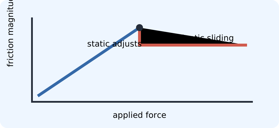
Static friction applies when the contacting surfaces do not slide relative to one another. The word static describes the contact, not necessarily the whole object. A rolling tire can have a momentarily stationary contact patch and therefore experience static friction while the vehicle moves. Static friction adjusts over a range to prevent slipping when possible. Its magnitude is not automatically at its maximum.

The empirical condition is $0\le f_s\le\mu_sN$. The symbol $f_s$ is static-friction magnitude, $\mu_s$ is the dimensionless coefficient of static friction, and $N$ is normal-force magnitude. The upper limit $f_{s,\max}=\mu_sN$ applies at impending slip. Below that threshold, Newton’s laws determine the particular friction needed. Writing $f_s=\mu_sN$ before establishing impending motion is a common modeling error.

Kinetic friction applies when the two surfaces slide relative to one another. A common introductory model is $f_k=\mu_kN$, where $f_k$ is kinetic-friction magnitude and $\mu_k$ is the dimensionless kinetic coefficient. Often $\mu_k<\mu_s$, so maintaining sliding requires less friction than initiating it. This equation is an empirical approximation whose accuracy depends on materials, surface conditions, speed range, temperature, and other factors. It is not a fundamental force law valid for every contact.

Understand the normal force

The normal force is the perpendicular contact force exerted by a surface. The word normal means perpendicular in geometry. It is not automatically equal to weight $mg$. Its value is found from Newton’s second law in the direction perpendicular to the contact. Friction models then use that determined value of $N$.

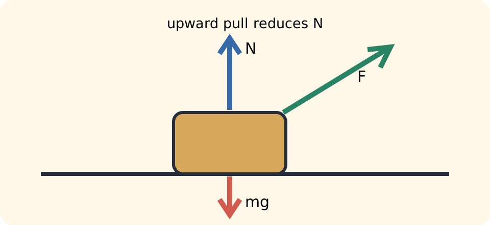
For an object on a horizontal surface with no vertical acceleration and no other vertical forces, $N-mg=0$, so $N=mg$. If a person pulls upward at angle $\theta$, the vertical component $F\sin\theta$ reduces the required normal force: $N=mg-F\sin\theta$. If the person pushes downward, the applied vertical component increases $N$. The component angle must be measured from the horizontal for this sine expression. Because friction scales with $N$ in the empirical model, pull angle can affect horizontal resistance.

On an incline of angle $\theta$, weight resolves into $mg\sin\theta$ parallel to the slope and $mg\cos\theta$ perpendicular to it. When there is no perpendicular acceleration and no other perpendicular force, $N=mg\cos\theta$. This is smaller than $mg$ for a nonzero incline angle. Substituting $mg$ directly into friction on a slope would therefore overestimate it. Component equations must precede the friction calculation.

Analyze a horizontal threshold

Consider a $10.0\,\mathrm{kg}$ crate on a horizontal floor with $\mu_s=0.400$ and $\mu_k=0.300$. Using $g=9.81\,\mathrm{\dfrac{m}{s^2}}$, vertical equilibrium gives $N=mg=(10.0\,\mathrm{kg})(9.81\,\mathrm{\dfrac{m}{s^2}})=98.1\,\mathrm{N}$. The maximum static friction is $f_{s,\max}=(0.400)(98.1\,\mathrm{N})=39.2\,\mathrm{N}$. The coefficient contributes no unit because it is a ratio of force magnitudes. This value is a limit, not the current friction in every resting case.

If a horizontal force of $30.0\,\mathrm{N}$ is applied, the crate can remain at rest because the required opposing static friction is only $30.0\,\mathrm{N}$. The net horizontal force is zero and acceleration is $0\,\mathrm{\dfrac{m}{s^2}}$. Friction does not rise to $39.2\,\mathrm{N}$ because that would create an unbalanced force in the opposite direction. Static friction matches the applied tendency up to its limit. The inequality contains this adjusting behavior.

If the applied force reaches $50.0\,\mathrm{N}$, static friction cannot maintain rest because $50.0\,\mathrm{N}>39.2\,\mathrm{N}$. Once sliding begins, the kinetic model gives $f_k=(0.300)(98.1\,\mathrm{N})=29.4\,\mathrm{N}$. The net force is $50.0\,\mathrm{N}-29.4\,\mathrm{N}=20.6\,\mathrm{N}$. Acceleration is $a=\dfrac{20.6\,\mathrm{N}}{10.0\,\mathrm{kg}}=2.06\,\mathrm{\dfrac{m}{s^2}}$ in the applied-force direction. The change from static to kinetic contact changes the governing force value.

Solve impending motion on an incline

Place a block at rest on an incline of angle $\theta$. Gravity’s parallel component $mg\sin\theta$ tends to make it slide down the slope. Static friction therefore points up the slope while equilibrium remains possible. The perpendicular equation gives $N=mg\cos\theta$. The required static friction is $f_s=mg\sin\theta$.

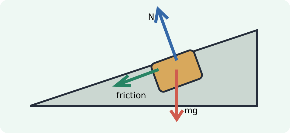
At the threshold of downward slipping, required friction equals its maximum. Thus $mg\sin\theta=\mu_smg\cos\theta$. Canceling $m$, $g$, and $\cos\theta$ gives $\tan\theta=\mu_s$. The threshold angle is called an angle of repose in some contexts. Its independence from mass follows because both the downslope demand and normal-force-based capacity scale with $mg$.

Suppose $\mu_s=0.500$. The threshold angle is $\theta=\tan^{-1}(0.500)=26.6^\circ$. At $20.0^\circ$, static friction is below its maximum and exactly balances $mg\sin20.0^\circ$. At $30.0^\circ$, the required value exceeds the static limit, so the block begins sliding under the model. A solution that assigns $f_s=\mu_sN$ at $20.0^\circ$ would falsely predict a nonzero net force up the incline.

Analyze sliding on an incline

Once a block slides down an incline, kinetic friction points up the incline. Choosing downhill as positive gives $mg\sin\theta-f_k=ma$. With $f_k=\mu_kmg\cos\theta$, cancellation of mass gives $a=g(\sin\theta-\mu_k\cos\theta)$. The result assumes an ideal constant coefficient and no other along-slope forces. It also assumes contact remains intact.

For $\theta=30.0^\circ$, $\mu_k=0.200$, and $g=9.81\,\mathrm{\dfrac{m}{s^2}}$, acceleration is $a=(9.81\,\mathrm{\dfrac{m}{s^2}})[\sin30.0^\circ-(0.200)\cos30.0^\circ]=3.21\,\mathrm{\dfrac{m}{s^2}}$ downhill. The trigonometric functions are dimensionless. Mass cancels because both weight components and kinetic friction scale with it. The calculated acceleration is smaller than frictionless $g\sin30.0^\circ=4.91\,\mathrm{\dfrac{m}{s^2}}$, as expected. Friction has reduced but not reversed the downhill acceleration.

If an object is sliding up the incline, kinetic friction points down the incline because that opposes relative sliding. Gravity’s parallel component also points down. The acceleration is therefore downhill even while velocity is uphill, causing the object to slow. After it stops, the contact must be reclassified; static friction may hold it or it may slide down. Friction direction can change when the motion tendency changes.

Use friction in circular motion

On a flat curve, static friction can supply the inward net force needed for a vehicle to turn. The radial equation is $f_s=m\dfrac{v^2}{r}$ as long as the tires do not slip. Because $f_s\le\mu_sN$ and $N=mg$ on a level road, the no-slip condition is $m\dfrac{v^2}{r}\le\mu_smg$. Canceling mass gives $v\le\sqrt{\mu_sgr}$. This is a limit, not a statement that friction always equals its maximum during every turn.

If the vehicle travels more slowly than the threshold, static friction adopts the smaller value needed for that speed. Doubling speed at fixed radius multiplies the required friction by four. Wet or icy conditions reduce the available coefficient and therefore reduce the maximum safe speed. Increasing curve radius lowers the force requirement at a given speed. These relationships explain why tight, fast turns are demanding.

The friction force points toward the center even though the vehicle’s velocity is tangent to the curve. It prevents the tire contact patch from sliding sideways relative to the road. If available friction is insufficient, the vehicle follows a path with less curvature than intended rather than being pushed radially outward by a new real force. In an inertial frame, loss of inward force leaves velocity changing too slowly in direction. Careful frame language prevents “centrifugal force” from being inserted into the free-body diagram without explanation.

Understand rolling without slipping

Rolling without slipping satisfies $v_{\mathrm{cm}}=\omega R$, where $v_{\mathrm{cm}}$ is center-of-mass speed, $\omega$ is angular speed, and $R$ is radius. The point of contact is instantaneously at rest relative to the surface. Friction at that contact is therefore static, not kinetic. Static friction may be zero, forward, or backward depending on applied torques and acceleration constraints. Rolling motion cannot be analyzed with the rule that friction always opposes center-of-mass velocity.

For a driven wheel, engine torque tends to make the tire push backward on the road. The road responds with forward static friction on the tire, accelerating the vehicle. For a freely rolling wheel pulled at its axle, friction may point backward to create the torque required for angular acceleration. The direction is found by predicting relative slip without friction. Rotational dynamics completes the quantitative analysis.

Rolling resistance in real systems is distinct from ideal static friction. Tire and surface deformation, internal hysteresis, and microscopic losses create resistance even without gross sliding. It is often modeled with an effective force or torque rather than $\mu_kN$. Bearings and air drag introduce further losses. “Rolling without slipping” removes kinetic sliding at the contact but does not guarantee zero energy dissipation in a real vehicle.

Connect work and energy transfer

Kinetic friction often decreases an object’s mechanical energy. For a block sliding distance $d$ on a fixed horizontal surface, friction does work $W_f=-f_kd$ when force opposes displacement. The negative sign indicates energy leaves the modeled translational kinetic-energy account. It may appear as increased internal energy of the block, surface, and surroundings. Energy is transformed rather than destroyed.

The thermal energy increase associated with two surfaces sliding relative to each other can be modeled as $\Delta E_{\mathrm{th}}=f_kd_{\mathrm{rel}}$ under simple conditions. The distance $d_{\mathrm{rel}}$ is the relative sliding distance at the contact. This system-level account avoids assigning all generated thermal energy to only one object without evidence. Sound, wear, and deformation may also receive energy. The selected system boundary determines which transfers are internal and which cross the boundary.

Static friction can do positive, negative, or zero work on an individual object depending on the motion of its contact point in the chosen frame. In ideal rolling on a stationary surface, the instantaneous contact point has zero velocity, so ideal static friction may do no work at that instant. On a moving conveyor belt, static friction can increase a package’s kinetic energy. Slogans that friction always removes mechanical energy are therefore too broad. Work depends on force and displacement of the point where the force acts.

Develop a microscopic model

Surfaces that appear smooth contain microscopic high points called asperities. Actual contact occurs over a much smaller area than the apparent geometric area. Local deformation brings atoms close enough for electromagnetic adhesion and bond formation. Sliding requires repeated deformation, shearing, and bond breaking. These processes produce resistance and internal-energy change.

Increasing normal force generally enlarges real microscopic contact area and strengthens aggregate interactions. This helps motivate the approximate proportionality $f\propto N$ for many dry surfaces over limited ranges. The near-independence from apparent contact area in the elementary model does not mean geometry never matters. Soft materials, lubricants, roughness, speed, temperature, contamination, and wear can change behavior. Coefficients summarize experimental conditions rather than immutable material constants.

At the atomic level, friction is electromagnetic, even though it is categorized as a mechanical contact force macroscopically. The normal force also arises from electromagnetic interactions resisting interpenetration. A coefficient model hides enormous microscopic complexity inside a simple measured ratio. That simplification is valuable when its limits are respected. More advanced tribology studies the detailed science of friction, lubrication, and wear.

Measure coefficients experimentally

One method slowly increases a horizontal pulling force on an object. The largest force recorded just before motion begins estimates $f_{s,\max}$. If the pull is horizontal and vertical acceleration is zero, $N=mg$, so $\mu_s=\dfrac{f_{s,\max}}{N}$. During steady-speed sliding, net horizontal force is zero and the measured pull estimates $f_k$. Then $\mu_k=\dfrac{f_k}{N}$ under the simple model.

An incline method increases angle until the object just begins to slide. The threshold relation $\mu_s=\tan\theta_c$ estimates the static coefficient. During downhill sliding with measured acceleration $a$, the equation $a=g(\sin\theta-\mu_k\cos\theta)$ can be solved for $\mu_k$. Angle and acceleration uncertainty propagate into the coefficient estimate. Multiple trials should be reported rather than one threshold observation.

Experimental coefficients depend on surface pair and condition. Reporting “the coefficient of wood” is incomplete because wood-on-wood, wood-on-metal, dry, wet, polished, and rough contacts differ. Cleanliness and wear may change across trials. A good report names both materials, preparation, loading range, speed range, method, and uncertainty. Empirical parameters carry the history of how they were measured.

Repair common mistakes

The most common mistake is setting $f_s=\mu_sN$ for every static situation. The correct statement is $f_s\le\mu_sN$, with equality only at impending slip. First solve the force balance for required static friction. Then compare that value with the maximum. If the requirement exceeds the limit, the static assumption fails and motion changes.

Another mistake is assuming $N=mg$. This equality holds only under particular perpendicular-force and acceleration conditions. Inclines, angled pulls, elevators, curved paths, and additional loads change the normal force. Write the perpendicular component of Newton’s second law. Only then substitute $N$ into a friction model.

A third mistake is directing friction opposite an object’s ground velocity. Friction opposes relative sliding or impending sliding between the surfaces at contact. Walking, driven wheels, and conveyor belts provide counterexamples. Temporarily remove friction and predict which way the contact surfaces would slip relative to one another. Restore friction opposite that tendency on the object being analyzed.

Practice with full reasoning

A stationary crate requires $12.0\,\mathrm{N}$ of friction to balance an applied push, while its maximum static friction is $20.0\,\mathrm{N}$. The actual static friction is $12.0\,\mathrm{N}$ opposite the impending slide. It is not $20.0\,\mathrm{N}$ because the maximum is only an available limit. Net force remains zero. Explain how the value would change as the push gradually increased to $18.0\,\mathrm{N}$.

A $5.00\,\mathrm{kg}$ sled slides on level ground with $\mu_k=0.250$. The normal force is $N=(5.00\,\mathrm{kg})(9.81\,\mathrm{\dfrac{m}{s^2}})=49.1\,\mathrm{N}$ to three significant figures. Kinetic friction is $f_k=(0.250)(49.1\,\mathrm{N})=12.3\,\mathrm{N}$. If friction is the only horizontal force, acceleration magnitude is $a=\dfrac{12.3\,\mathrm{N}}{5.00\,\mathrm{kg}}=2.45\,\mathrm{\dfrac{m}{s^2}}$. Its direction is opposite relative sliding.

A $20.0\,\mathrm{kg}$ crate is pulled with $100\,\mathrm{N}$ at $30.0^\circ$ above horizontal on a surface with $\mu_k=0.200$. Vertical equilibrium gives $N=(20.0\,\mathrm{kg})(9.81\,\mathrm{\dfrac{m}{s^2}})-(100\,\mathrm{N})\sin30.0^\circ=146\,\mathrm{N}$. Kinetic friction is $29.2\,\mathrm{N}$. Horizontal net force is $(100\,\mathrm{N})\cos30.0^\circ-29.2\,\mathrm{N}=57.4\,\mathrm{N}$, giving $a=2.87\,\mathrm{\dfrac{m}{s^2}}$. Compare this with a horizontal pull and explain how the upward component affects both normal force and friction.

Consolidate the contact model

Friction is determined by contact kinematics and force balance. Static friction adjusts according to $0\le f_s\le\mu_sN$, while kinetic friction is often approximated by $f_k=\mu_kN$. The normal force must be solved from perpendicular dynamics and is not universally $mg$. Direction opposes relative sliding or its tendency at the contact. These principles replace unreliable slogans with a repeatable method.

The workflow is to select the object, draw all real forces, choose axes, predict slip tendency, assign friction direction, solve perpendicular dynamics for $N$, and test the static threshold. If slipping occurs, change to the kinetic model and solve the new motion. Check units, signs, acceleration direction, and limiting cases. Compare the required static value with its maximum before deciding that motion begins. Treat the static and kinetic states as distinct models connected by a threshold.

Friction also links mechanics to energy and materials science. Macroscopic resistance emerges from microscopic deformation, adhesion, and bond processes. Mechanical energy can become internal energy, sound, wear, or other forms while total energy remains accounted for. Coefficients are empirical and condition-dependent. Understanding those layers prepares you to analyze work, rolling, machines, vehicles, and real experimental surfaces with appropriate caution.