Quadratic Functions Model Curved Change

A linear function changes by a constant amount over equal input intervals, but many relationships bend because their rate of change itself changes. The height of a projectile, the area enclosed by a variable rectangle, and the stopping distance of a vehicle can all involve quadratic structure under suitable models. A quadratic function is a polynomial function of degree two, commonly written $f(x)=ax^2+bx+c$ with $a\ne0$. The condition $a\ne0$ ensures that the squared term is present; otherwise the expression would be linear or constant. Its graph is a parabola whose algebraic forms reveal different geometric features.

Understanding quadratics requires more than memorizing a formula for roots. The coefficients, zeros, vertex, axis of symmetry, intercepts, and rate pattern are multiple descriptions of one function. Moving deliberately among standard, factored, and vertex forms allows the representation to match the question. Each transformation must preserve equality even though the visible expression changes. The goal is to see these forms as coordinated lenses rather than unrelated procedures.

We will begin with tables and differences, then connect them to the parabola’s symmetry. We will interpret the three principal algebraic forms, derive vertex information by completing the square, solve for zeros, and use the discriminant to classify roots. We will also examine transformations and modeling constraints. Throughout, symbols will be defined and conclusions will be checked in more than one representation.

Constant second differences reveal quadratic structure

Suppose a table uses equally spaced input values. First differences subtract consecutive output values, while second differences subtract consecutive first differences. A linear function has constant first differences because its slope is constant. A quadratic function has constant second differences because its first differences change linearly. This diagnostic depends on equal input spacing and should not be applied blindly to irregularly spaced data.

Consider $f(x)=x^2$ at $x=0,1,2,3,4$. The outputs are $0,1,4,9,16$. The first differences are $1,3,5,7$, which are not constant but increase by two each time. The second differences are therefore $2,2,2$, which are constant. The changing first differences express the graph’s curvature.

For $f(x)=ax^2+bx+c$ sampled with input step one, the constant second difference is $2a$. The coefficient $b$ affects the first-difference level but not its successive change, and $c$ shifts every output without affecting either difference pattern. If the input step is $h$ instead, the second difference becomes $2ah^2$. This relationship connects a numerical table directly to the leading coefficient. It also provides a check when fitting a quadratic through data.

A parabola has a turning point and an axis of symmetry

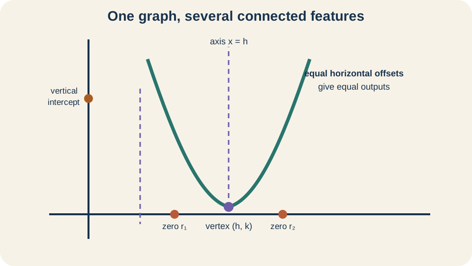
The graph of every real quadratic function is a parabola. It opens upward when $a>0$ and downward when $a<0$. An upward-opening parabola has a minimum point, while a downward-opening parabola has a maximum point. That turning point is called the vertex. The vertical line through the vertex is the axis of symmetry.

If the vertex is $(h,k)$, the axis is $x=h$. Points equally far left and right of this axis have equal function values. Algebraically, vertex form makes this visible because $(x-h)^2$ has the same value when $x=h-r$ or $x=h+r$. Both substitutions produce $r^2$. Symmetry reduces graphing work and connects paired zeros.

The domain of a quadratic polynomial is all real numbers because every real $x$ can be squared, multiplied, and added. Its range depends on the vertex and opening direction. If $a>0$, then $f(x)\ge k$, so the range begins at the minimum $k$. If $a<0$, then $f(x)\le k$, so the range ends at the maximum $k$. A real-world model may impose a narrower practical domain than the algebraic function.

Standard form emphasizes coefficients and the vertical intercept

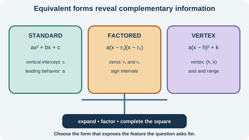
Standard form is $f(x)=ax^2+bx+c$, where $a$, $b$, and $c$ are real constants and $a\ne0$. Substituting $x=0$ gives $f(0)=c$, so the graph crosses the vertical axis at $(0,c)$. The leading coefficient $a$ controls opening direction and vertical scale. The coefficient $b$ helps locate the axis of symmetry. Together, the three coefficients determine the entire parabola.

The axis of symmetry in standard form is $x=-\frac{b}{2a}$. The horizontal fraction bar means $-b$ is divided by the product $2a$. Substituting this input into the function gives the vertex’s vertical coordinate. Thus the vertex is $\left(-\frac{b}{2a},f\left(-\frac{b}{2a}\right)\right)$. This relationship will be derived by completing the square rather than accepted as an isolated rule.

For $f(x)=2x^2-8x+3$, the vertical intercept is $(0,3)$. The axis is $x=-\frac{-8}{2(2)}=2$. Substituting gives $f(2)=2(4)-8(2)+3=-5$, so the vertex is $(2,-5)$. Because $a=2>0$, this vertex is the global minimum. The standard-form coefficients have therefore supplied both an intercept and the symmetry location.

Factored form emphasizes zeros and sign changes

Factored form is $f(x)=a(x-r_1)(x-r_2)$ when the quadratic has real zeros $r_1$ and $r_2$. A zero is an input where $f(x)=0$, corresponding to a horizontal-axis intercept. The zero-product property says a product equals zero when at least one factor equals zero. Therefore $x=r_1$ and $x=r_2$ are zeros. The leading factor $a$ retains opening and scale information.

The axis of symmetry lies halfway between two real zeros. Its horizontal coordinate is $h=\frac{r_1+r_2}{2}$. This midpoint follows from the mirror symmetry of the parabola. Substituting $h$ into $f$ gives the vertex height. If the two zeros coincide, the parabola touches the axis at its vertex rather than crossing it.

For $f(x)=x^2-6x+5$, factoring gives $f(x)=(x-1)(x-5)$. The zeros are $1$ and $5$, and their midpoint is $\frac{1+5}{2}=3$. Evaluating $f(3)$ gives $9-18+5=-4$, so the vertex is $(3,-4)$. The function is negative between its zeros and positive outside them because the two factors have opposite signs only in the middle interval. A sign table verifies those interval conclusions systematically.

Vertex form emphasizes transformations and extrema

Vertex form is $f(x)=a(x-h)^2+k$. The vertex is $(h,k)$ and the axis of symmetry is $x=h$. The expression $(x-h)^2$ is never negative for real $x$. Consequently, if $a>0$, the smallest function value is $k$, while if $a<0$, the largest function value is $k$. This form makes optimization conclusions nearly immediate.

The signs inside and outside the square have different visual effects. Replacing $x$ by $x-h$ shifts the parent graph $y=x^2$ horizontally by $h$ units, with positive $h$ shifting right. Adding $k$ shifts the graph vertically by $k$ units. Multiplying by $a$ reflects the graph across the horizontal axis when $a<0$ and changes vertical scale by $|a|$. These transformations alter location and shape while preserving parabolic symmetry.

For $f(x)=-2(x+1)^2+8$, rewrite $x+1$ as $x-(-1)$ to identify $h=-1$. The vertex is $(-1,8)$ and the axis is $x=-1$. Because $a=-2$, the graph opens downward and has maximum value $8$. The magnitude $|a|=2$ makes vertical output differences twice those of the parent parabola at corresponding horizontal offsets. Substitution of symmetric inputs such as $-2$ and $0$ confirms equal outputs.

Completing the square converts standard form to vertex form

Completing the square rewrites a quadratic expression by creating a perfect-square trinomial. The identity $x^2+bx=\left(x+\frac{b}{2}\right)^2-\left(\frac{b}{2}\right)^2$ preserves equality because the added square and subtracted square cancel. Expanding the first square gives $x^2+bx+\frac{b^2}{4}$. Subtracting $\frac{b^2}{4}$ leaves the original expression. The method is therefore controlled addition of zero.

For $x^2-6x+5$, take half of $-6$, which is $-3$, and square it to obtain $9$. Write $x^2-6x+5=(x^2-6x+9)-9+5$. The trinomial becomes $(x-3)^2$, and the constants combine to $-4$. Thus $x^2-6x+5=(x-3)^2-4$. Equality can be checked by expanding the result.

For a leading coefficient other than one, factor it from the quadratic and linear terms first. Starting with $ax^2+bx+c$, write $a\left(x^2+\frac{b}{a}x\right)+c$. Completing the square inside produces $a\left(x+\frac{b}{2a}\right)^2+c-\frac{b^2}{4a}$. The squared factor reveals $h=-\frac{b}{2a}$. This derivation explains the axis formula and identifies the vertex height as $c-\frac{b^2}{4a}$.

Solving a quadratic means locating zeros

Solving $ax^2+bx+c=0$ asks for inputs where the quadratic function has output zero. Factoring is efficient when a product form can be recognized. Completing the square is systematic and supports geometric interpretation. The quadratic formula works for every quadratic with $a\ne0$. Graphing estimates real roots visually but should not substitute for exact algebra when exact values are required.

The quadratic formula is $x=\frac{-b\pm\sqrt{b^2-4ac}}{2a}$. The symbol $\pm$ means two cases, one using addition and one using subtraction. The radical covers the entire discriminant $b^2-4ac$, while the horizontal fraction bar divides the entire numerator by $2a$. Parentheses are essential when substituting negative coefficients. The formula follows from completing the square on the general equation.

Apply it to $2x^2-8x+3=0$. Here $a=2$, $b=-8$, and $c=3$, giving $x=\frac{8\pm\sqrt{64-24}}{4}=\frac{8\pm\sqrt{40}}{4}$. Since $\sqrt{40}=2\sqrt{10}$, the roots simplify to $x=2\pm\frac{\sqrt{10}}{2}$. Their midpoint is $2$, matching the previously calculated axis. Substitution or symmetry checks the result. Both signs must be evaluated to obtain the complete solution set.

The discriminant classifies root behavior

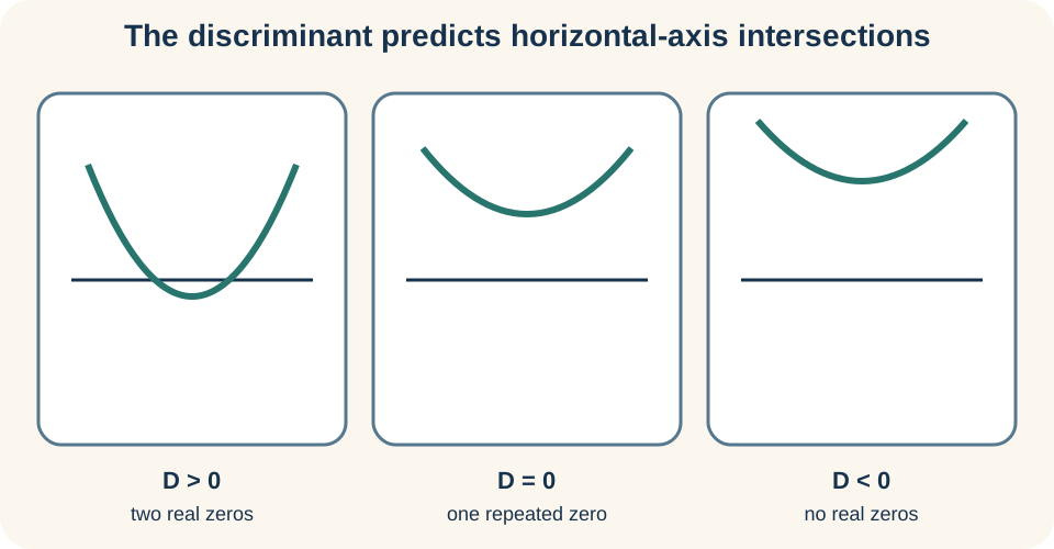
The discriminant is $D=b^2-4ac$, the quantity under the square root in the quadratic formula. If $D>0$, its positive square root produces two distinct real roots. If $D=0$, both formula branches give the same real root. If $D<0$, no real number has the required negative square, so the roots are a complex-conjugate pair. The discriminant predicts type before the roots are fully calculated.

The graph reflects these cases. Two real roots mean the parabola crosses the horizontal axis twice. One repeated real root means the vertex touches the axis. No real roots means the parabola stays entirely above the axis when it opens upward or entirely below when it opens downward. This geometry provides an independent interpretation of the algebraic sign.

The discriminant also relates directly to vertex height. In the completed-square form of $ax^2+bx+c$, the vertex height is $-\frac{D}{4a}$. If $a>0$ and $D<0$, this value is positive, so an upward-opening parabola never reaches zero. If $a>0$ and $D>0$, the vertex is negative and the graph crosses twice. The relationship unifies formula, vertex, and graph.

Intercepts, sign intervals, and end behavior build a graph

A reliable sketch begins with the opening direction, axis, vertex, and intercepts. The vertical intercept comes from $f(0)=c$ in standard form. Horizontal intercepts come from solving $f(x)=0$ when real roots exist. Symmetry supplies a reflected point across the axis. End behavior follows the leading term because $ax^2$ dominates for large $|x|$.

When $a>0$, both ends of the graph rise as $x\to\infty$ and $x\to-\infty$. When $a<0$, both ends fall. The notation $x\to\infty$ means $x$ increases without bound, while $x\to-\infty$ means it decreases without bound. Lower-degree terms become small relative to $ax^2$ at large magnitude. End behavior is therefore controlled by the sign of $a$.

Real zeros partition the number line into sign intervals. In $a(x-r_1)(x-r_2)$ with $r_1<r_2$, test the signs of each factor in the three intervals. A simple root changes the sign of one factor and therefore changes the product sign. A repeated root has even multiplicity and does not change sign. This analysis supports inequalities as well as graphing.

Transformations are best read from vertex form

Start with the parent function $p(x)=x^2$. The function $p(x-h)$ shifts its graph horizontally because the same parent input occurs when $x$ is $h$ units larger. This inside transformation can feel backward until it is checked with the vertex. Setting $x-h=0$ gives $x=h$, so the turning point moves to horizontal coordinate $h$. Substitution resolves sign confusion more reliably than a slogan.

The outside operations are more direct. Multiplying by $a$ multiplies every output, creating a vertical stretch when $|a|>1$ and a vertical compression when $0<|a|<1$. A negative $a$ also reflects every output across the horizontal axis. Adding $k$ then shifts each output by $k$. The order follows the expression’s function composition.

To graph $g(x)=\frac{1}{2}(x-4)^2-3$, begin at vertex $(4,-3)$. It opens upward because $\frac{1}{2}>0$ and is vertically compressed relative to $y=x^2$. One unit left or right of the vertex produces an output increase of $\frac{1}{2}$. Two units away produces an increase of $\frac{1}{2}(4)=2$. Symmetric point construction makes the scale visible.

Quadratic models require a meaningful domain

Suppose a projectile-height model is $h(t)=-4.9t^2+20t+1.5$, where $h$ is measured in meters and time $t$ in seconds. The negative leading coefficient represents downward curvature under a constant-gravity approximation. The model’s vertex estimates maximum height and its positive zero estimates ground impact. A negative-time root may be algebraically valid but irrelevant if the model begins at release. Physical interpretation restricts the domain to a relevant interval.

Units clarify coefficient meaning. The term $-4.9t^2$ must have meters, so its coefficient carries units $\frac{\mathrm{m}}{\mathrm{s^2}}$. The coefficient $20$ carries $\frac{\mathrm{m}}{\mathrm{s}}$, and the constant $1.5$ carries meters. Every term then has the same output unit and may be added. A number such as $4.9$ without units hides the dimensional logic.

Quadratic regression can fit curved data, but a good fit does not prove the mechanism is quadratic outside the observed range. Extrapolation may predict impossible negative lengths, unrealistic growth, or behavior beyond the model’s assumptions. Residuals, measurement uncertainty, and domain knowledge should accompany the fitted coefficients. The algebra describes the model exactly, while the model describes reality only approximately. Keep those two claims distinct.

Optimization uses the vertex with constraints

Many elementary optimization problems reduce to a quadratic. If a rectangle has fixed perimeter $P$, let one side be $x$ and the other be $\frac{P}{2}-x$. Its area is $A(x)=x\left(\frac{P}{2}-x\right)=-x^2+\frac{P}{2}x$. The leading coefficient is negative, so the vertex gives a maximum. The physically meaningful domain is $0<x<\frac{P}{2}$.

Using $h=-\frac{b}{2a}$ with $a=-1$ and $b=\frac{P}{2}$ gives $x=\frac{P}{4}$. The other side is also $\frac{P}{4}$, so the maximum-area rectangle is a square. This conclusion follows from the quadratic model plus the domain constraint. Endpoints would give zero area and confirm the interior vertex is preferable. Units of area are squared length units.

Optimization requires naming what is varied, what is fixed, and what quantity is optimized. A vertex outside the feasible domain is not the practical solution. If the domain is a closed interval, compare the vertex when included and both endpoints. If only integer inputs are permitted, evaluate nearby integers around a noninteger vertex. Algebra supplies candidates, while constraints determine admissibility.

Common errors and corrective checks

One error is reading $h$ directly from the visible sign in $(x-h)^2$. In $(x+3)^2$, rewrite the factor as $(x-(-3))^2$, so $h=-3$. Another error is treating $c$ as the vertex height in standard form. The constant $c$ is the vertical intercept, and it equals the vertex height only in special cases. Substitution resolves both misunderstandings.

A second error is dividing only one term by $2a$ in the quadratic formula. The horizontal fraction bar groups the entire numerator $-b\pm\sqrt{b^2-4ac}$. Use parentheses during substitution, especially when $b$ is negative. A third error is forgetting to factor $a$ before completing the square. The half-and-square step applies to the coefficient of $x$ after the squared term has coefficient one inside the grouping.

A strong final check compares representations. Expand factored or vertex form to recover standard coefficients. Substitute each proposed root into the original equation. Confirm that two roots have midpoint $-\frac{b}{2a}$ and that the vertex matches the opening direction. For models, check units and the practical domain. Independent agreement is better evidence than a repeated calculation.

A connected example across all three forms

Start with $f(x)=x^2-6x+5$. Standard form immediately gives the vertical intercept $(0,5)$ and upward opening because $a=1>0$. Factoring gives $(x-1)(x-5)$, so the zeros are $1$ and $5$. Completing the square gives $(x-3)^2-4$, so the vertex is $(3,-4)$. The same function has not changed; only the visible information has.

The zeros’ midpoint is $3$, matching the axis from vertex form and the formula $-\frac{-6}{2(1)}=3$. The vertex height $-4$ is negative, so an upward-opening graph must cross the axis twice. The discriminant is $(-6)^2-4(1)(5)=16>0$, confirming two distinct real roots. Substitution of $x=1$ and $x=5$ gives zero in the original expression. These cross-checks form a network rather than a one-way procedure.

Choose the form according to the question. Standard form is convenient for the vertical intercept and coefficient comparison. Factored form is convenient for zeros and sign intervals. Vertex form is convenient for extrema, axis, transformations, and range. Fluency means converting when necessary rather than forcing every question through one representation.

Retrieval and connection forward

Without looking back, define a quadratic function and explain why $a\ne0$. Describe constant second differences, the vertex, axis of symmetry, and how the sign of $a$ controls opening. State what standard, factored, and vertex forms reveal most directly. Then derive $h=-\frac{b}{2a}$ by completing the square in outline. If a formula cannot be explained in words, revisit its construction.

Quadratic equations lead naturally to the quadratic formula, complex roots, and polynomial factorization. Their graphs support inequality solving because zeros divide sign intervals. In calculus, the vertex corresponds to a point where instantaneous rate of change is zero, and the constant second derivative reflects fixed curvature. In statistics, quadratic regression extends linear modeling while raising stronger extrapolation concerns. The same structure therefore connects foundational algebra to later mathematics and science.

The enduring insight is representational choice. A quadratic is one function with several equivalent algebraic faces, and each face makes different evidence easy to see. Tables reveal second differences, graphs reveal symmetry, factors reveal zeros, and completed squares reveal extrema. Equivalence allows movement among them without changing the underlying relationship. That movement is the real skill behind quadratic reasoning.