Graphing Linear Relationships

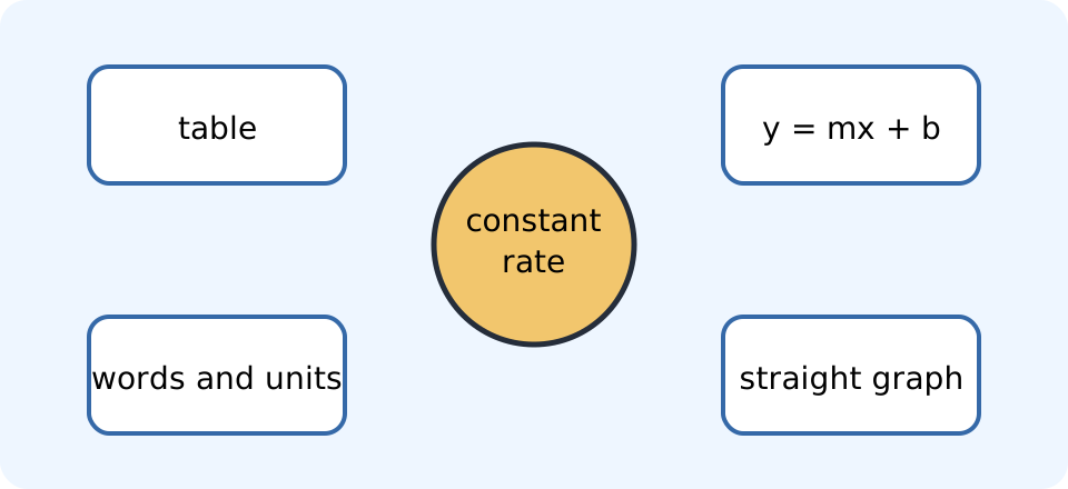
A linear relationship has a constant rate of change. Its table, equation, graph, and verbal description are not separate topics; they are different representations of the same structure. Slope measures the constant rate, an intercept anchors the relationship at a reference input, and a line displays all allowed input-output pairs geometrically. Units and context determine what those mathematical features mean. This lesson develops a method for moving deliberately among representations, checking results, and recognizing when a straight-line model stops being credible.

Build meaning into the coordinate plane

A coordinate graph places paired values on perpendicular axes. The horizontal axis usually represents an input variable $x$, while the vertical axis usually represents an output variable $y$. An ordered pair $(x,y)$ lists the horizontal coordinate first and the vertical coordinate second. The point $(3,7)$ therefore means input $3$ is paired with output $7$. Axis labels and units are necessary to turn those numbers into a meaningful statement.

The origin is $(0,0)$, where both coordinates equal zero. Positive $x$ values lie to the right and negative $x$ values lie to the left under the standard orientation. Positive $y$ values lie above and negative $y$ values lie below. The plane is divided into four quadrants, but points on an axis belong to no quadrant. These conventions create a shared spatial language for algebraic relationships.

A graph is not automatically a picture of a physical path. If $x$ is time in seconds and $y$ is temperature in degrees Celsius, the line shows temperature change over time rather than an object traveling uphill. Its geometry encodes numerical relationships. Before interpreting shape, ask what each axis measures and which units it uses. Context translates position on the page back into meaning.

Recognize constant rate in a table

A relationship is linear when equal input changes produce equal output changes over its domain. In a table, calculate $\dfrac{\Delta y}{\Delta x}$ between pairs of rows. The delta symbol means final value minus initial value. If this ratio is constant for every interval, the data lie exactly on a nonvertical line. Unequal input spacing is acceptable as long as each output change is compared with its corresponding input change.

Consider pairs $(0,5)$, $(2,11)$, $(5,20)$, and $(9,32)$. The first ratio is $\dfrac{11-5}{2-0}=3$, the second is $\dfrac{20-11}{5-2}=3$, and the third is $\dfrac{32-20}{9-5}=3$. Because the rate remains three output units per input unit, the relationship is linear. Simply comparing output differences would have been misleading because the input intervals are not equal. Rate standardizes change by the amount of input change.

Measured data rarely produce perfectly identical ratios because of noise and limited precision. A line may still be an appropriate approximation when rates vary slightly without a systematic pattern. Plotting the data helps reveal curvature, clusters, and unusual points. Regression methods can estimate a best-fitting line, but the resulting line does not make the underlying relationship exactly linear. Model language should distinguish exact algebraic structure from empirical approximation.

Define slope as a rate of change

Between distinct points $(x_1,y_1)$ and $(x_2,y_2)$, slope is $m=\dfrac{y_2-y_1}{x_2-x_1}=\dfrac{\Delta y}{\Delta x}$. The symbol $m$ conventionally denotes slope. The denominator must be nonzero because division by zero is undefined. Interchanging point order changes both numerator and denominator signs, leaving the ratio unchanged. Reversing only one difference incorrectly reverses the slope.

Slope units are output units per input unit. If volume $V$ in litres is graphed against time $t$ in minutes, slope units are $\mathrm{\dfrac{L}{min}}$. A slope of $-4.00\,\mathrm{\dfrac{L}{min}}$ means volume decreases by $4.00\,\mathrm{L}$ for each additional minute. It does not mean the container holds a negative volume. The sign reports direction of change, while magnitude reports sensitivity.

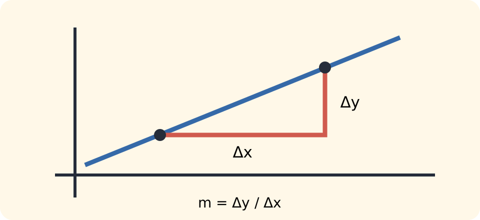
Positive slope means output increases as input increases, negative slope means output decreases, and zero slope means output remains constant. A larger absolute slope produces more output change per input unit. Visual steepness alone can be misleading because graph scales can differ. The numerical ratio with units is the stable description. On an exact line, any two distinct points yield the same slope.

Derive slope–intercept form

Suppose a relationship has constant slope $m$ and output $b$ when input is zero. Starting at the point $(0,b)$, changing input by $x$ changes output by $mx$. Adding that change to the starting output gives $y=mx+b$. This is slope–intercept form. The coefficient $m$ is slope and the constant $b$ is the vertical or $y$-intercept.

The intercept is the output associated with $x=0$. It may represent an initial amount, base charge, calibration offset, or another reference value. Calling it an initial value is appropriate only when zero input corresponds to the beginning of the modeled process. If zero lies outside the meaningful domain, $b$ may be an algebraic extrapolation without direct physical interpretation. Context decides whether the intercept is observable.

For $y=-2x+6$, begin with $(0,6)$. A slope of $-2=\dfrac{-2}{1}$ means move one unit right and two units down to reach another point such as $(1,4)$. Repeating reaches $(2,2)$ and $(3,0)$. Drawing the unique line through these points represents every real input-output pair allowed by the algebra. A contextual domain may restrict which portion of that line is meaningful.

Build a line from a point and slope

When one point $(x_1,y_1)$ and slope $m$ are known, point–slope form is $y-y_1=m(x-x_1)$. The differences $y-y_1$ and $x-x_1$ measure changes from the known point to an arbitrary point $(x,y)$ on the line. Their ratio equals $m$. This form keeps the given information visible. It avoids solving for the vertical intercept before writing an equation.

Suppose a line has slope $5$ and passes through $(2,-1)$. Point–slope form gives $y-(-1)=5(x-2)$, or $y+1=5(x-2)$. Expanding yields $y+1=5x-10$, so $y=5x-11$. Substituting $(2,-1)$ gives $-1=10-11$, verifying the point. The coefficient of $x$ remains $5$, verifying the slope.

Point–slope form works especially well with measured baselines that are not located at input zero. A temperature might be known at noon with a steady rate afterward, or a reservoir might have a measured volume at day ten. Writing change from that reference can preserve interpretation. Conversion to slope–intercept form is optional unless another task benefits from it. Equivalent forms describe the same set of points.

Build a line from two points

Two points with different $x$ coordinates determine one nonvertical line. First calculate $m=\dfrac{y_2-y_1}{x_2-x_1}$. Then use either point in $y-y_1=m(x-x_1)$. Algebraic simplification can produce slope–intercept or standard form. Substitution of both original points verifies that no arithmetic error changed the line.

For points $(2,5)$ and $(6,13)$, slope is $m=\dfrac{13-5}{6-2}=\dfrac84=2$. Using $(2,5)$ gives $y-5=2(x-2)$. Expanding produces $y=2x+1$. Substitution gives $5=2(2)+1$ and $13=2(6)+1$. Both checks succeed.

If the points share an $x$ coordinate, the denominator is zero and the line is vertical. Its equation is $x=c$, where $c$ is that shared coordinate. It cannot be written as $y=mx+b$ because one input $x=c$ is paired with many $y$ values. The undefined slope is a consequence of division by zero, not merely an arbitrary label. Recognizing the special case before calculation prevents an invalid fraction.

Use standard form and intercepts

Standard form is often written $Ax+By=C$, where $A$, $B$, and $C$ are constants. It treats the variables more symmetrically and can be convenient for systems of equations. To expose slope, solve for $y$ when $B\ne0$. Rearranging gives $y=-\dfrac{A}{B}x+\dfrac{C}{B}$. Thus slope is $-\dfrac{A}{B}$ and vertical intercept is $\dfrac{C}{B}$.

An $x$-intercept occurs where $y=0$, because points on the horizontal axis have zero vertical coordinate. A $y$-intercept occurs where $x=0$. For $2x+3y=12$, setting $y=0$ gives $x=6$, so the $x$-intercept is $(6,0)$. Setting $x=0$ gives $y=4$, so the $y$-intercept is $(0,4)$. Two distinct intercepts can be used to graph the line efficiently.

Converting the same equation gives $3y=-2x+12$ and $y=-\dfrac23x+4$. This exposes slope $-\dfrac23$ and confirms vertical intercept $4$. From $(0,4)$, move three units right and two units down to reach $(3,2)$ and then $(6,0)$. The intercept method and slope-step method produce the same geometry. Multiple representations cross-check one another.

Translate a contextual model

A linear model often has the structure output equals initial amount plus rate times input. A tank containing $180\,\mathrm{L}$ drains at $6.00\,\mathrm{\dfrac{L}{min}}$. If $t$ is elapsed time in minutes and $V(t)$ is volume in litres, the model is $V(t)=180\,\mathrm{L}-(6.00\,\mathrm{\dfrac{L}{min}})t$. Multiplying the rate by minutes produces litres. Both terms can therefore be combined dimensionally.

The intercept $180\,\mathrm{L}$ is the volume at $t=0\,\mathrm{min}$. The slope is negative because the volume decreases by $6.00\,\mathrm{L}$ each minute. Setting $V=0\,\mathrm{L}$ gives $t=30.0\,\mathrm{min}$. The physically meaningful domain is $0\,\mathrm{min}\le t\le30.0\,\mathrm{min}$ under the assumptions. Extending the line later predicts negative liquid volume and therefore breaks the model.

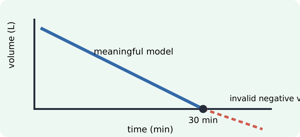
Model construction should identify variables, units, signs, domain, and assumptions. Constant slope assumes the drain rate does not change as the tank empties. In a real unregulated outlet, pressure and flow rate may decrease with liquid height. The linear relation may still approximate a limited interval. A model is a purposeful representation, not a claim that reality remains straight forever.

Interpret temperature conversion

Fahrenheit temperature $F$ and Celsius temperature $C$ are related by $F(C)=\dfrac95C+32$. The slope $\dfrac95=1.8$ means a change of $1\,^{\circ}\mathrm{C}$ corresponds to a change of $1.8\,^{\circ}\mathrm{F}$. The intercept says $0\,^{\circ}\mathrm{C}$ corresponds to $32\,^{\circ}\mathrm{F}$. These are temperature-scale coordinates rather than thermal-energy ratios. The offset means one cannot convert absolute readings by multiplying alone.

At $C=20.0\,^{\circ}\mathrm{C}$, substitution gives $F=(\dfrac95)(20.0)+32=68.0\,^{\circ}\mathrm{F}$. The input unit is degrees Celsius and output unit is degrees Fahrenheit. A temperature interval of $10.0\,^{\circ}\mathrm{C}$ corresponds to $18.0\,^{\circ}\mathrm{F}$, but an absolute reading of $10.0\,^{\circ}\mathrm{C}$ corresponds to $50.0\,^{\circ}\mathrm{F}$. Distinguishing changes from coordinates explains the role of the intercept. The model’s units belong with its variables and coefficients.

Solving for Celsius gives $C=\dfrac59(F-32)$. This inverse relationship undoes the original conversion. Its slope $\dfrac59$ is the reciprocal of $\dfrac95$, as expected when input and output roles reverse. The subtraction of $32$ must occur before scaling. Composing the two conversion functions returns the original temperature coordinate and verifies the algebra.

Understand horizontal, vertical, parallel, and perpendicular lines

A horizontal line has equation $y=c$ for constant $c$. Any two points on it have $\Delta y=0$, so slope is zero. Its graph is a function of $x$ because each input has exactly one output. In context, it represents an output that does not change with input. Zero slope is a defined rate, not an undefined one.

A vertical line has equation $x=c$. Any two distinct points on it have $\Delta x=0$, so the slope ratio would divide by zero and is undefined. It fails the vertical-line test for a function $y$ of $x$ because input $c$ corresponds to many outputs. Its direction remains perfectly well defined even though its slope number does not. It can still represent a valid geometric relation. “Not a function of $x$” does not mean “not mathematically meaningful.”

Parallel nonvertical lines have equal slopes. Perpendicular nonvertical lines with nonzero slopes satisfy $m_1m_2=-1$, so their slopes are negative reciprocals. A line perpendicular to slope $\dfrac23$ has slope $-\dfrac32$. Horizontal and vertical lines form the exceptional perpendicular pair. These relationships follow from direction geometry rather than graph appearance alone.

Graph with a deliberate strategy

To graph from slope–intercept form, plot $(0,b)$ and use the slope ratio to locate at least one additional point. To graph from standard form, intercepts may be fastest. To graph from a table, plot several pairs and check their alignment. To graph from a point and slope, begin at the known point rather than searching for $b$. Strategy should match the information already available.

Label axes with variable names and units. Choose a scale that includes the relevant domain and makes meaningful differences visible. Use evenly spaced tick marks for an ordinary linear axis and state clearly if a transformation is used. Mark whether points are discrete or form a continuous interval. Connecting isolated categories or integer-only possibilities with an unbroken line can falsely imply allowed intermediate values.

After drawing, verify the graph against the equation. Check the intercept, slope sign, and at least one additional point. Ask whether the line occupies the correct quadrants and respects contextual domain restrictions. A graphing utility can render an entered equation flawlessly even when the equation was modeled incorrectly. Visual output is evidence only after its inputs and interpretation are checked.

Read graph scale ethically

Changing the axis scale changes apparent steepness without changing numerical slope. A line can look nearly horizontal when the vertical range is broad or extremely steep when the vertical range is narrow. Slope calculations use coordinate values and remain unchanged. Readers should inspect tick spacing before comparing visual rates. Graph geometry communicates through its scale.

A truncated vertical axis can magnify small differences. Truncation is not automatically deceptive when the goal is to show small but important variation, but it must be clear. Including zero can sometimes hide meaningful local structure, while omitting zero can exaggerate practical importance. The choice should follow the question and be disclosed. Multiple views may be appropriate when both absolute magnitude and fine variation matter.

Unequal aspect ratios can make perpendicular lines look nonperpendicular on screen. Responsive layouts may resize a plot differently on desktop and mobile. Mathematical interpretation should rely on labeled coordinates rather than pixel angle alone. Accessible graphs also use text, patterns, or markers rather than color as the only distinction. A graph is a measurement instrument and should be designed with the care expected of one.

Distinguish interpolation and extrapolation

Interpolation predicts between observed input values. Extrapolation predicts outside the observed range. Both use the fitted relationship, but extrapolation relies more heavily on the assumption that the same structure continues into unobserved conditions. A straight pattern over a short interval may curve, saturate, or reach a physical boundary later. Distance beyond the data matters.

Suppose cost data are observed for production from $100$ to $500$ units. A linear estimate at $300$ units is interpolation, while an estimate at $10{,}000$ units is distant extrapolation. Bulk discounts, capacity limits, or new equipment may alter the rate. The algebraic line remains defined, but empirical support does not extend automatically. Model domain is an evidentiary concept as well as an algebraic one.

Negative contextual predictions are common warnings. A population, volume, mass, or price model may eventually cross zero and continue negative. The line has not made an arithmetic mistake; the assumptions have exceeded their useful range. State a restricted domain or replace the model with one that includes relevant constraints. Interpretation decides where the mathematics applies.

Repair common mistakes

A common slope error reverses the order in only one difference. If the numerator is $y_2-y_1$, the denominator must be $x_2-x_1$. Reversing both produces an equivalent ratio. Draw a slope triangle and associate vertical change with the same direction of horizontal travel. This links signs to geometry rather than memory.

Another error drops units from slope. A bare value such as $12$ is incomplete when it actually means $12\,\mathrm{\dfrac{m^3}{h}}$ or $12\,\mathrm{\dfrac{dollars}{item}}$. Units identify which quantity changes per unit of which other quantity. They can also reveal reversed axes because reciprocal units signal a reciprocal rate. Write units inside numerical substitutions and final interpretations.

A third error treats the intercept as universally meaningful and the graph as unlimited. Input zero may lie outside the domain, and distant inputs may violate constant-rate assumptions. Check what zero means in context and mark the evidence-supported interval. Do not confuse an equation’s infinite mathematical line with a model’s finite practical reach. Graphing is complete only when domain and scale are interpreted.

Practice across representations

Find the slope through $(-1,4)$ and $(3,-8)$. Using consistent order gives $m=\dfrac{-8-4}{3-(-1)}=\dfrac{-12}{4}=-3$. Point–slope form using $(-1,4)$ is $y-4=-3(x+1)$. Simplification gives $y=-3x+1$. Substitute both points to verify the result.

Find both intercepts of $3x+2y=12$. Setting $y=0$ gives $x=4$, so one intercept is $(4,0)$. Setting $x=0$ gives $y=6$, so the other is $(0,6)$. Solving for $y$ gives $y=-\dfrac32x+6$. Use the slope to verify that moving two units right from $(0,6)$ moves three units down to $(2,3)$.

A reservoir begins with $250\,\mathrm{m^3}$ and fills at $12.0\,\mathrm{\dfrac{m^3}{h}}$. Its model is $V(t)=250\,\mathrm{m^3}+(12.0\,\mathrm{\dfrac{m^3}{h}})t$ for a justified time domain. The intercept represents initial volume, and the slope represents volume gained per hour. At $5.00\,\mathrm{h}$, volume is $310\,\mathrm{m^3}$. Name at least two real conditions that could eventually invalidate the constant-rate assumption.

Consolidate the linear framework

A linear relationship has constant rate of change. Slope $m=\dfrac{\Delta y}{\Delta x}$ quantifies that rate with output-per-input units. Slope–intercept form $y=mx+b$ displays rate and zero-input output. Point–slope form $y-y_1=m(x-x_1)$ emphasizes a known point and rate. Standard form $Ax+By=C$ often makes intercepts and systems convenient.

Tables show repeated rates, equations encode rules, graphs display geometry, and words provide context. Moving among them creates checks that no single representation supplies alone. Intercepts, signs, scales, domains, and units all carry meaning. Horizontal and vertical lines require special attention, and parallel or perpendicular slopes express direction relationships. A correct line is more than marks on a coordinate plane.

Linear models are powerful because constant change is understandable and often useful over limited ranges. Their simplicity also makes unsupported extrapolation tempting. Ask what evidence supports the rate, what zero means, which inputs are allowed, and how graph design shapes perception. These questions turn graphing from a mechanical plotting exercise into mathematical modeling. The same habits will guide systems, inequalities, rates of change, data fitting, and calculus.