Sequences Use Position to Organize Values

A sequence is an ordered collection of values, and the order is part of its mathematical identity. The same numbers arranged differently form a different sequence because each position carries meaning. Sequence notation provides a compact way to name individual terms, describe how terms depend on position, and express how one term generates another. This framework appears in population models, payment schedules, computer algorithms, numerical approximations, and infinite-series theory. Learning it begins with treating the index as an input rather than as decoration.

You will learn to interpret $a_n$, specify an index set, compare explicit and recursive definitions, derive arithmetic and geometric formulas, use finite differences and ratios diagnostically, and translate between lists, tables, graphs, and rules. You will also study shifted indices, partial sums, recurrence iteration, and modeling limits. Every subscript, exponent, and ellipsis will be explained. Examples will distinguish a term’s position from its value. The goal is to reason about sequences as functions on discrete domains.

Begin any sequence problem by identifying the first allowed index and pairing each displayed value with its index. Determine whether the rule gives a term directly or depends on earlier terms. Test a proposed formula on the initial term and at least two later terms. State the domain because a rule beginning at $n=0$ can describe a shifted list relative to the same formula beginning at $n=1$. Finally, treat a pattern inferred from finite data as a model rather than a logically unique conclusion.

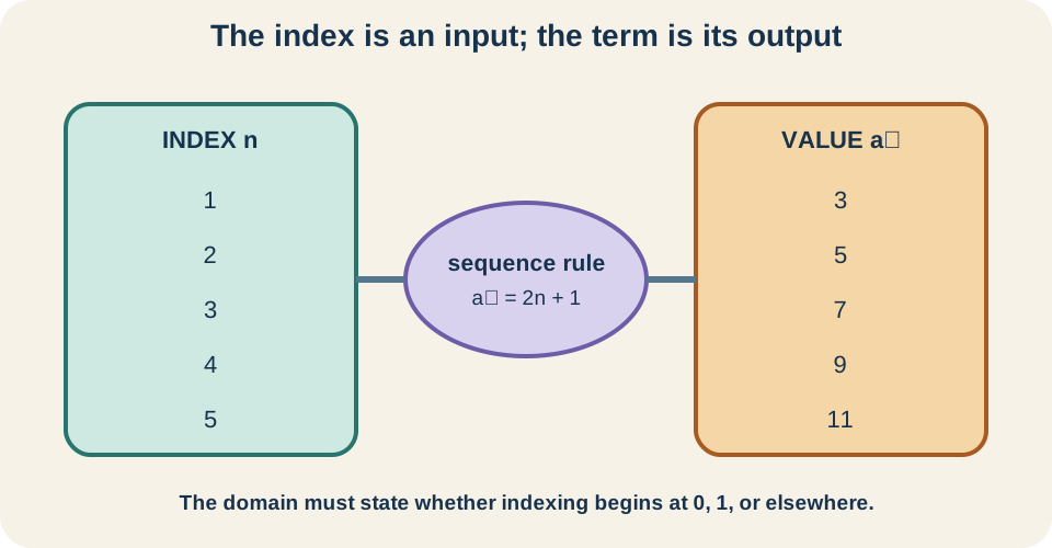
A sequence is a function with an ordered discrete domain

A function assigns exactly one output to each allowed input. A sequence is a function whose domain is an ordered set of integers, often $1,2,3,\ldots$ or $0,1,2,\ldots$. The values may be real numbers, complex numbers, vectors, functions, or other mathematical objects. Ordering comes from the index domain rather than from the numerical sizes of the outputs. A sequence may increase, decrease, repeat, or behave irregularly while remaining well defined.

The notation $a_n$ is read “a sub n” and means the term of sequence $a$ at index $n$. The subscript $n$ labels an input; it is not multiplication by $n$. Thus $a_5$ means the value in position five when indexing begins at one, while $5a$ would indicate multiplication in a different context. A full sequence may be denoted $\{a_n\}$ together with its index range. Braces here refer to the family of indexed terms, though precise contexts distinguish sequences from unordered sets.

For the list $3,5,7,9,\ldots$ indexed from one, $a_1=3$, $a_2=5$, and $a_4=9$. The ellipsis indicates continuation but does not, by itself, uniquely define how continuation occurs. A formula such as $a_n=2n+1$ makes the intended rule explicit for positive integers $n$. Substituting $n=1$ gives $3$, and substituting $n=4$ gives $9$. The index-to-value mapping is now unambiguous.

The starting index is part of the definition

The formula $a_n=2^n$ gives different first displayed values depending on its domain. If $n=1,2,3,\ldots$, the sequence begins $2,4,8,\ldots$. If $n=0,1,2,\ldots$, it begins $1,2,4,8,\ldots$. The algebraic expression has not changed, but the allowed inputs have. A sequence definition is incomplete when its index set is ambiguous.

Different fields use different starting conventions. Introductory sequences often begin at one because “first term” naturally corresponds to $a_1$. Computer science frequently begins indexing at zero, making the first stored element $a_0$. Power series naturally use $n=0$ because the constant term contains $x^0$. Neither convention is universally correct; consistency and explicitness matter.

Reindexing shifts labels without necessarily changing the ordered values. If $a_n=2^n$ for $n\ge0$, define $b_n=a_{n-1}$ for $n\ge1$. Then $b_1=a_0=1$, $b_2=a_1=2$, and the displayed values match while the labels differ. The expression for $b_n$ is $2^{n-1}$. Shifted exponents often arise because of this index translation.

Explicit rules compute terms directly

An explicit rule expresses $a_n$ using the index $n$ and fixed parameters without requiring earlier sequence values. For $a_n=3+2(n-1)$, substituting any allowed positive integer gives the corresponding term directly. To find $a_{100}$, calculate $3+2(99)=201$. No preceding ninety-nine terms need to be generated. Explicit formulas are therefore efficient for distant-term evaluation.

The expression $n-1$ counts the number of steps from index one to index $n$. At $n=1$, zero steps have occurred, so the formula returns the starting value $3$. At $n=2$, one increment of two has occurred, giving $5$. At $n=100$, ninety-nine increments have occurred. This step-count interpretation is more reliable than memorizing the visible pattern.

An explicit rule also clarifies domain restrictions. The expression $a_n=\frac{1}{n-3}$ is undefined at $n=3$, so a claimed domain containing three would fail unless that term is separately defined. The expression $a_n=\sqrt{n-5}$ requires $n\ge5$ for real values. A sequence domain can skip or begin after problematic integers. Formula and domain jointly define the function.

Recursive rules describe generation from prior terms

A recursive definition gives one or more initial values and a rule connecting later terms to earlier ones. The sequence $3,5,7,9,\ldots$ can be defined by $a_1=3$ and $a_{n+1}=a_n+2$ for $n\ge1$. The first statement supplies a starting anchor. The second says the next term equals the current term plus two. Both parts are necessary.

The notation $a_{n+1}$ means the term whose index is one greater than $n$. It does not mean $a_n+1$. When $n=1$, the recurrence gives $a_2=a_1+2=5$. When $n=2$, it gives $a_3=a_2+2=7$. Repeated substitution generates the list step by step.

Recursive descriptions emphasize local dynamics and often mirror real processes. A bank balance next month may depend on this month’s balance, interest, deposits, and withdrawals. A population next year may depend on the current population through a growth rule. Computer algorithms can compute recurrence terms iteratively without a closed form. The tradeoff is that reaching a distant term may require all intervening terms unless an explicit solution is found.

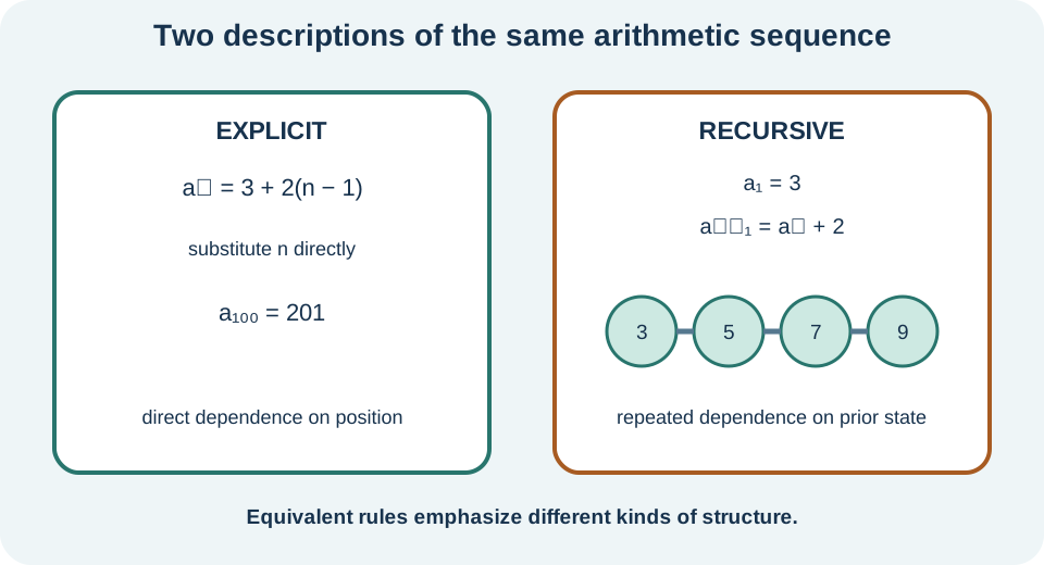
Arithmetic sequences have constant first difference

An arithmetic sequence changes by a constant amount $d$ from one term to the next. The recursive definition is $a_{n+1}=a_n+d$. Subtracting consecutive terms gives $a_{n+1}-a_n=d$, which explains the phrase common difference. The value $d$ may be positive, negative, or zero. Equal index steps produce equal output changes.

If the first term is $a_1$, then reaching $a_n$ requires $n-1$ increments of $d$. The explicit formula is $a_n=a_1+(n-1)d$. At $n=1$, the added part is zero and the formula returns the initial term. At $n=2$, one difference is added. This initial-term check guards against the common off-by-one error.

For $10,7,4,1,\ldots$, the common difference is $d=-3$. With $a_1=10$, the explicit rule is $a_n=10-3(n-1)$. Expanding gives $a_n=13-3n$, an equivalent formula. Substitution of $n=1$ and $n=4$ reproduces $10$ and $1$, confirming both initial placement and step size. The negative difference explains why the terms decrease as the index grows.

Geometric sequences have constant ratio

A geometric sequence multiplies by a constant ratio $r$ from one term to the next. Its recursive form is $a_{n+1}=ra_n$. When terms are nonzero, dividing consecutive terms gives $\frac{a_{n+1}}{a_n}=r$. The ratio can produce growth, decay, sign alternation, or a constant sequence depending on its value. Multiplication replaces the repeated addition of an arithmetic sequence.

Starting from $a_1$, reaching term $a_n$ requires $n-1$ multiplications by $r$. The explicit formula is $a_n=a_1r^{n-1}$. The exponent $n-1$ counts repeated multiplications, just as the arithmetic factor $n-1$ counts repeated additions. At $n=1$, $r^0=1$, so the formula returns $a_1$. The zero exponent is essential to the starting-index convention.

For $5,15,45,135,\ldots$, the common ratio is $r=3$. The recursive definition is $a_1=5$ and $a_{n+1}=3a_n$. The explicit rule is $a_n=5\cdot3^{n-1}$. Then $a_4=5\cdot3^3=135$. Both representations describe the same sequence from different viewpoints.

Differences and ratios diagnose but do not prove a rule

Computing first differences is a useful diagnostic for arithmetic structure. Constant first differences across a table support an arithmetic model. Constant second differences support a quadratic model when indices are equally spaced. Higher finite differences can reveal polynomial patterns of higher degree. These tests organize evidence from discrete values.

Computing consecutive ratios similarly tests a geometric model. If $\frac{a_{n+1}}{a_n}$ is constant wherever denominators are nonzero, the observed terms follow geometric behavior. Ratios are undefined when a denominator term is zero, so the test needs care. Rounding in measured data may make ratios approximately rather than exactly constant. A model may then be fitted and evaluated rather than declared exact.

No finite list determines a unique infinite continuation without additional assumptions. The first values $1,2,3,4$ suggest $a_n=n$, but another formula can agree for those indices and diverge later. For example, adding a term that contains $(n-1)(n-2)(n-3)(n-4)$ changes later values while leaving the first four untouched. Pattern recognition is therefore an inference based on simplicity or context. State the assumed model class when uniqueness matters.

Graphs of sequences are discrete point sets

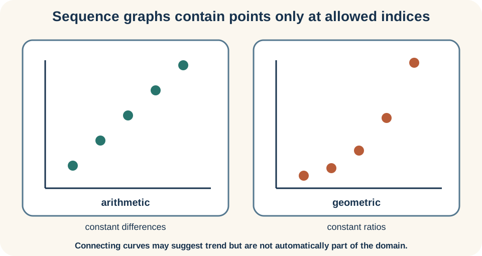
Graph a sequence by plotting ordered pairs $(n,a_n)$ for allowed indices. Because the domain is discrete, the graph consists of separate points rather than a continuous curve. Connecting points may help the eye see a trend, but the connecting segments are not automatically part of the sequence. An input such as $n=2.5$ may have no sequence value. The graph should preserve that domain distinction.

An arithmetic sequence produces points lying on a line because $a_n=a_1+(n-1)d$ is linear in $n$. The slope of the supporting line is $d$. A geometric sequence produces points following an exponential shape when $r>0$, because the index appears in an exponent. The continuous exponential curve can interpolate the pattern, but it defines an extension beyond the original sequence. Discrete and continuous models answer different input questions.

Plotting can expose indexing mistakes. If the first term should appear at $n=1$ but the formula places it at $n=0$, every point is shifted horizontally. A table with columns labeled $n$ and $a_n$ provides a direct pre-graph check. Axes should name the index and the term’s units when applicable. Position is usually dimensionless, while outputs may carry dollars, meters, organisms, or another unit.

Recursive and explicit forms can be converted

For an arithmetic recurrence $a_{n+1}=a_n+d$, repeated substitution gives $a_2=a_1+d$, $a_3=a_1+2d$, and $a_4=a_1+3d$. The coefficient of $d$ is always one less than the index. Generalizing gives $a_n=a_1+(n-1)d$. This derivation links local repeated change to global position. The explicit form is not a separate fact but a compressed recurrence history.

For a geometric recurrence $a_{n+1}=ra_n$, repeated substitution gives $a_2=ra_1$, $a_3=r^2a_1$, and $a_4=r^3a_1$. Again the exponent is one less than the index. Generalizing gives $a_n=a_1r^{n-1}$. Induction can turn this observed structure into a proof for all positive integers. The base case and update rule mirror the recursive definition.

Not every recurrence has a simple elementary explicit formula. The Fibonacci sequence, defined by $F_0=0$, $F_1=1$, and $F_{n+2}=F_{n+1}+F_n$, depends on two earlier terms. It has a closed form, but the recurrence is often more natural computationally and conceptually. Other recurrences may require matrix methods, generating functions, or numerical iteration. Explicit and recursive are forms of description, not rankings of mathematical legitimacy.

Partial sums create a new sequence

Given a sequence $a_1,a_2,a_3,\ldots$, define its $n$th partial sum by $S_n=\sum_{k=1}^{n}a_k$. The capital sigma $\sum$ directs repeated addition. The index $k$ is a temporary summation variable that begins at one and ends at $n$. Thus $S_3=a_1+a_2+a_3$. The partial sums $S_1,S_2,S_3,\ldots$ form a new sequence.

For an arithmetic sequence with first term $a_1$ and last included term $a_n$, the finite sum is $S_n=\frac{n(a_1+a_n)}{2}$. The horizontal fraction bar divides the product $n(a_1+a_n)$ by two. This formula reflects pairing first with last, second with next-to-last, and so on. An equivalent form substitutes $a_n=a_1+(n-1)d$. Both require knowing exactly how many terms are included.

For a geometric sequence with first term $a_1$ and ratio $r\ne1$, the finite sum is $S_n=a_1\frac{1-r^n}{1-r}$. The exponent $n$ counts the number of included terms through the cancellation derivation. When $r=1$, every term equals $a_1$ and the sum is simply $na_1$, so the displayed fraction’s zero denominator signals a separate case. Partial sums lead directly toward infinite-series convergence. Finite and infinite sums must not be conflated.

Growth and decay models use ratios with units and time steps

A repeated percent change produces geometric structure when each period uses the same multiplicative factor. A growth rate of $5\%$ per period corresponds to factor $1+0.05=1.05$. If $P_0$ is the initial amount at index zero, then $P_n=P_0(1.05)^n$. Here $n$ counts completed periods. The indexing convention aligns the zero index with zero elapsed periods.

A decay rate of $12\%$ per period leaves $88\%$, so the factor is $0.88$, not $-0.12$. The model becomes $A_n=A_0(0.88)^n$. Outputs remain positive when $A_0>0$, while decreasing toward zero. The phrase “decrease by twelve percent” describes multiplying the previous amount by one minus the decimal rate. Additive subtraction of a fixed amount would instead be arithmetic.

Units and period length belong to the ratio. A factor of $1.05$ per year cannot be applied for twelve monthly steps without converting the model. If compounding occurs monthly, a monthly factor must be supplied or derived under stated assumptions. Real populations, prices, and balances may have changing rates and external inputs. A geometric sequence is a model whose constant-ratio assumption must be evaluated.

Recurrences can include input as well as multiplication

Many practical sequences combine accumulated state with a recurring addition. A savings balance might follow $B_{n+1}=(1+r)B_n+p$, where $r$ is the interest rate per period and $p$ is a fixed deposit made according to a stated timing convention. The previous balance is multiplied before the deposit is added in this version. Changing deposit timing changes the recurrence. Every symbol must be tied to an event order.

Iterating from $B_0=0$ gives $B_1=p$, $B_2=(1+r)p+p$, and $B_3=(1+r)^2p+(1+r)p+p$. A geometric sum appears because earlier deposits receive more growth periods. This connection converts a recurrence into an explicit formula under constant $r$ and $p$. The derivation also shows why blindly using a compound-interest formula can miscount payment timing. Writing the first several terms exposes that timing before symbols conceal it.

Units check the recurrence. Both $B_n$ and $p$ have currency units, while $r$ is dimensionless per stated period. The factor $1+r$ is dimensionless, so $(1+r)B_n$ remains currency and can be added to $p$. If terms with incompatible units appear, the model is malformed. Dimensional reasoning applies to discrete models as strongly as to physical equations.

Index shifts require careful substitution

Sequence formulas often appear with $n+1$, $n-1$, or a general shift $n+m$. To find $a_{n+1}$ from an explicit rule, replace every occurrence of $n$ with $n+1$. If $a_n=n^2-3n$, then $a_{n+1}=(n+1)^2-3(n+1)$. Expanding gives $n^2-n-2$. Replacing only one occurrence would be an inconsistent substitution.

To find a first difference symbolically, compute $a_{n+1}-a_n$. For $a_n=n^2$, this is $(n+1)^2-n^2=2n+1$. The result depends linearly on $n$, showing that first differences change. Taking another difference gives a constant two. This algebra connects the table-based difference pattern to the formula.

Index shifts also appear in recurrences to align initial conditions. A rule written $a_n=a_{n-1}+d$ for $n\ge2$ is equivalent to $a_{n+1}=a_n+d$ for $n\ge1$. The allowed $n$ values change with the notation so both rules begin by computing $a_2$ from $a_1$. State the valid index range beside the recurrence. Without it, the earliest required previous term may be undefined.

Common errors and corrective habits

One common error is confusing $a_n$ with $an$. Subscripts name indexed terms, while adjacent symbols generally indicate multiplication. Another is omitting the starting index, producing an off-by-one shift in formulas such as $a_1r^{n-1}$. Test the first allowed index before trusting a rule. The initial term should emerge without extra steps.

A second error is identifying a geometric sequence from constant differences or an arithmetic sequence from constant ratios. Write separate diagnostic columns and label the operation. A third error is assuming that a few terms prove a unique continuation. State whether the rule is given, derived under an arithmetic or geometric assumption, or merely conjectured. Mathematical honesty includes the basis for pattern selection.

Recursive definitions can fail when initial conditions are missing or insufficient. A two-step recurrence usually needs two starting values, while a one-step recurrence needs one. Check that every requested term can be generated from supplied data. For explicit rules, check domain restrictions and units. For graphs, preserve discrete points rather than silently filling every real input.

A connected example across representations

Consider the sequence $4,9,14,19,\ldots$ beginning at $n=1$. Consecutive differences are all five, so an arithmetic model is supported. The recursive form is $a_1=4$ and $a_{n+1}=a_n+5$. The explicit form is $a_n=4+5(n-1)=5n-1$. Substituting $n=1$ and $n=4$ checks the endpoints shown.

The graph consists of points $(1,4),(2,9),(3,14),(4,19),\ldots$ lying on the line $y=5x-1$. The continuous line helps reveal slope but includes inputs not belonging to the original positive-integer domain. The tenth term is $a_{10}=5(10)-1=49$. The sum of the first ten terms is $S_{10}=\frac{10(4+49)}{2}=265$. Each conclusion uses the representation that makes it simplest.

Now shift to zero-based indexing while preserving the displayed values. Define $b_0=4$ and $b_{n+1}=b_n+5$ for $n\ge0$. The explicit formula becomes $b_n=4+5n$. Then $b_9=49$, corresponding to the same physical tenth listed value as $a_{10}$. The difference between nine and ten is indexing, not sequence content.

Retrieval and connection forward

Without looking back, define a sequence as a function and explain why its domain is discrete. Distinguish index, term, explicit rule, recursive rule, initial condition, common difference, and common ratio. Derive the arithmetic and geometric explicit formulas by counting steps from the first term. Then explain why a finite pattern does not logically determine a unique infinite sequence. If your explanation relies only on visual continuation, return to the role of assumptions.

Sequences lead naturally to summation notation, finite-series formulas, and infinite-series convergence. Difference equations provide discrete analogues of differential equations, while recurrence relations underlie algorithms and dynamic models. Arithmetic sequences connect to linear functions, and geometric sequences connect to exponential functions. Partial sums introduce accumulation, a theme that later appears in integration. Index discipline continues through vectors, matrices, probability, and programming.

The enduring insight is that position is data. A sequence rule does not merely generate numbers; it assigns a value to each allowed integer input. Explicit forms reveal dependence on position, recursive forms reveal dependence on prior state, and graphs preserve the discreteness of the domain. Differences, ratios, and sums expose structure without erasing assumptions. Once indices are handled deliberately, sequence notation becomes a precise language for repeated change.