Systems of Linear Equations

A single linear equation in two variables describes many ordered pairs. A system asks which ordered pairs satisfy several equations at the same time. The word simultaneous is the heart of the idea. A value that satisfies one equation but not the other is not a system solution. Graphs represent the same requirement as a common intersection.

Systems appear whenever several constraints act on the same unknowns. A budget and a quantity requirement can determine two purchase amounts. Two motion descriptions can identify when objects meet. Chemical balances, electrical networks, and data models can produce larger systems. Algebraic methods preserve the constraints while transforming them into easier forms.

This lesson connects four representations: equations, graphs, tables, and matrices. Substitution will use one equation to replace a variable expression. Elimination will combine equations to cancel a variable. Row reduction will generalize those operations. Every method will classify the system and verify the resulting solution in the original equations.

Learning objectives and an opening prediction

After this lesson, you should explain a solution as a point satisfying every equation. You should solve two-variable systems by graphing, substitution, and elimination. You should classify systems as having one, none, or infinitely many solutions. You should represent systems with augmented matrices and valid row operations. You should also construct and evaluate systems from contextual constraints.

Consider $y=2x+1$ and $y=-x+7$. Predict whether they meet once, never, or infinitely often. Their slopes differ, so the lines are not parallel and meet at exactly one point. Setting their expressions for $y$ equal gives $2x+1=-x+7$. The intersection is therefore an algebraic equality of outputs.

Now compare $2x+y=5$ with $4x+2y=10$. Multiplying the first equation by two produces the second. They describe the same line, so every point on that line satisfies both. The system has infinitely many solutions. Two written equations do not guarantee two independent constraints.

A solution satisfies every constraint

For the system $\begin{cases}a_1x+b_1y=c_1\\a_2x+b_2y=c_2\end{cases}$, a solution is an ordered pair $(x,y)$ that makes both equations true. The coefficients $a_i$ and $b_i$ multiply the unknowns, while $c_i$ are constants. Subscripts label equations. The braces indicate that the equations are considered together. They do not mean multiplication.

Testing a candidate requires substitution into each original equation. If $(2,3)$ is proposed for $x+y=5$ and $2x-y=1$, the first gives $2+3=5$ and the second gives $4-3=1$. Both statements are true. Therefore the pair solves the system. Passing only one test would be insufficient.

The solution set can contain one point, no points, or infinitely many points for two linear equations in two variables. It cannot contain exactly two distinct points unless the lines coincide, in which case they share infinitely many. Two distinct straight lines intersect at most once. Geometry and algebra agree on these possibilities. Classification is part of the answer.

Graphing makes simultaneous truth visible

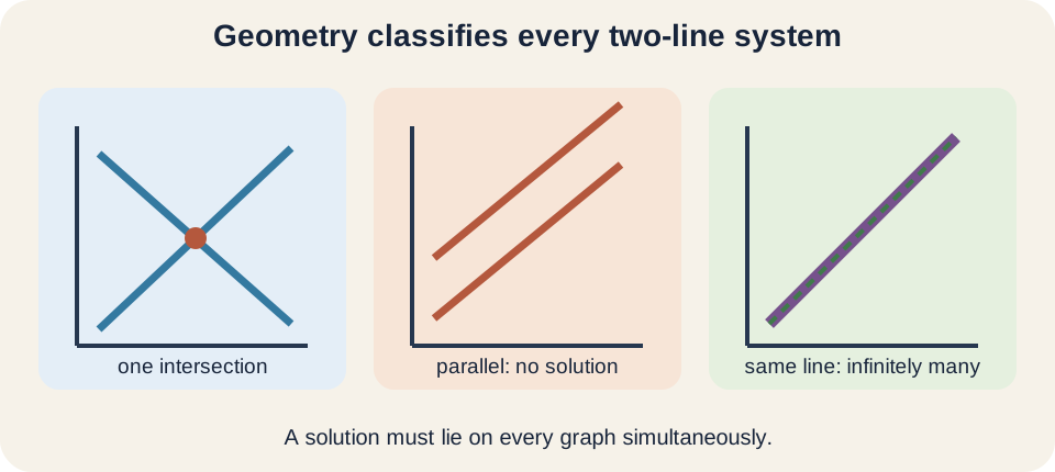
Each equation in two variables defines a line when it represents a nondegenerate linear relationship. Plot both lines on the same coordinate plane. Any intersection lies on both and therefore satisfies both equations. One crossing means one solution. Parallel distinct lines mean no solution, and coincident lines mean infinitely many.

Graphing is especially useful for estimation and interpretation. It reveals whether an algebraic answer is plausible and whether the intersection lies inside a meaningful domain. A contextual model may restrict $x$ and $y$ to nonnegative integers. A visible intersection outside that region can be algebraically valid yet contextually unusable. The graph makes constraints easier to see.

Graph accuracy is limited by scale and drawing resolution. An intersection near $(2.03,4.97)$ may look like $(2,5)$. Nearly parallel lines can place the intersection far outside the viewing window. Graphing technology can improve resolution but does not replace exact reasoning. Use graphs to understand structure and algebra to determine precise values.

Slope reveals solution count before solving

Write nonvertical lines as $y=m x+b$. The coefficient $m$ is slope and $b$ is vertical intercept. Different slopes imply one intersection. Equal slopes with different intercepts imply parallel lines and no solution. Equal slopes with equal intercepts imply the same line and infinitely many solutions.

Vertical lines require a separate form such as $x=k$. Two distinct vertical lines are parallel and have no intersection. A vertical line and a nonvertical line meet once. Slope-intercept classification still works conceptually, but vertical slope is undefined. Standard form avoids forcing every line into one notation.

Nearly equal slopes make a system sensitive. A small change in coefficients can move the intersection a large distance. This is not merely a graphing inconvenience. It is a form of numerical ill-conditioning. Later linear algebra will quantify sensitivity and stability.

Substitution replaces an equal expression

Substitution works best when one variable is already isolated or can be isolated simply. For $\begin{cases}y=2x+1\\x+y=7\end{cases}$, replace $y$ in the second equation with the equal expression $2x+1$. The result is $x+(2x+1)=7$. This one-variable equation preserves simultaneous truth. Every system solution must satisfy it.

Solve $3x+1=7$ to obtain $x=2$. Then return to either original relation, giving $y=2(2)+1=5$. The candidate is $(2,5)$. Verification gives $5=2(2)+1$ and $2+5=7$. Both equations hold.

Substitution is not the act of moving a symbol without justification. It relies on equality: if $y$ equals $2x+1$, either expression can replace the other in a valid context. Parentheses protect the substituted expression. If $y=-3x+4$, substituting into $2x-5y=1$ requires $2x-5(-3x+4)=1$. Omitting parentheses changes signs.

Worked substitution example with fractions

Solve $\begin{cases}3x-2y=7\\x=\frac{y+5}{2}\end{cases}$. Substitute the given expression for $x$ into the first equation: $3\left(\frac{y+5}{2}\right)-2y=7$. Multiply every term by two to clear the horizontal fraction: $3(y+5)-4y=14$. Expand to $3y+15-4y=14$. Then $-y=-1$, so $y=1$.

Use $x=\frac{y+5}{2}$ to find $x=\frac{1+5}{2}=3$. The candidate is $(3,1)$. Check the first equation: $3(3)-2(1)=9-2=7$. Check the second: $3=\frac{1+5}{2}=3$. The ordered pair satisfies both.

Clearing fractions is optional but often reduces arithmetic errors. Multiplying the entire equation by a nonzero number preserves its solution set. Multiplying only selected terms does not. Show the common factor across every term. The horizontal fraction bar makes numerator grouping explicit.

Elimination creates a zero coefficient

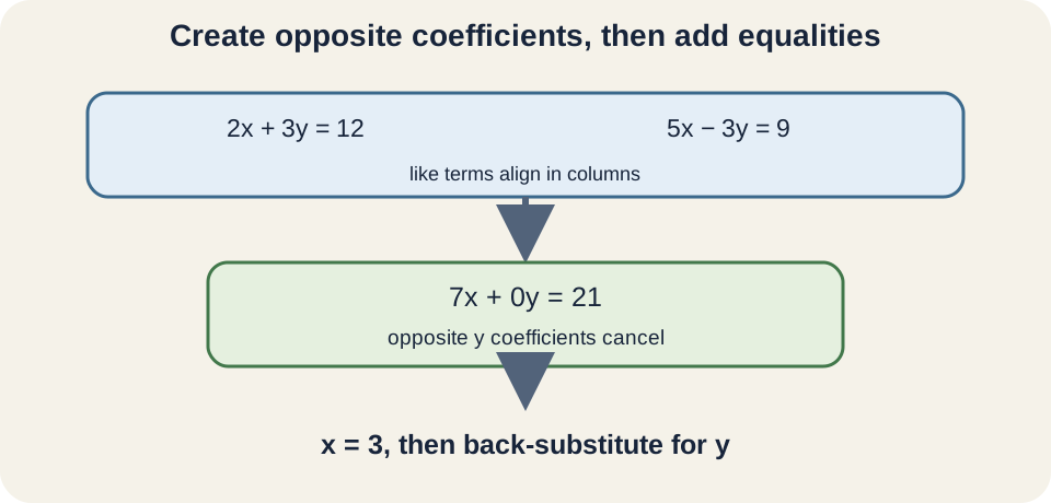
Elimination combines equations so one variable cancels. Adding equalities is valid: if left sides equal right sides separately, their sums are equal. Multiplying an entire equation by a nonzero constant is also valid. Choose multipliers that create opposite coefficients. Then add the transformed equations.

For $\begin{cases}2x+3y=12\\5x-3y=9\end{cases}$, the $y$ coefficients are already opposites. Add equations to obtain $7x=21$, so $x=3$. Substitute into the first equation: $6+3y=12$, hence $y=2$. The solution is $(3,2)$. Its coordinate order is always $(x,y)$.

Verification gives $2(3)+3(2)=12$ and $5(3)-3(2)=9$. Elimination produced one coordinate, but back-substitution produced the other. A single value such as $x=3$ is not the full two-variable solution. The second coordinate must remain paired with the first. Ordered-pair format preserves correspondence.

Choosing efficient multipliers

Suppose the system is $\begin{cases}3x+4y=11\\5x+6y=17\end{cases}$. To eliminate $x$, multiply the first equation by five and the second by negative three. The transformed equations are $15x+20y=55$ and $-15x-18y=-51$. Adding gives $2y=4$, so $y=2$. Substitution gives $x=1$.

One could instead eliminate $y$ using multipliers three and negative two. That creates $12y$ and $-12y$. Both routes are valid and should agree. Choose smaller least-common multiples when possible. Efficient arithmetic reduces, but never removes, the need for verification.

Scaling an equation changes its appearance but not its line. Every term, including the constant, must be multiplied. Multiplying $3x+4y=11$ by five gives $15x+20y=55$, not $15x+20y=11$. Failing to scale the constant creates a different line. Write transformed equations on separate rows to preserve bookkeeping.

Contradictions identify no solution

Consider $\begin{cases}2x+y=4\\4x+2y=11\end{cases}$. Multiply the first equation by negative two and add it to the second. The variables cancel, leaving $0=3$. This statement is false. Therefore no ordered pair satisfies both equations.

The contradiction reveals inconsistent constraints. Geometrically, the equations have equal slopes but different intercepts. Their coefficient rows are proportional while constants are not proportional. The lines are parallel and distinct. Algebra did not fail; it exposed incompatibility.

Do not attempt to divide by zero or invent a coordinate after obtaining a false statement. State “no solution” or use the symbol $\varnothing$ for the empty solution set. The symbol denotes a set containing no ordered pairs. In context, explain which requirements conflict. An impossible model may indicate incorrect data, assumptions, or transcription.

Identities identify dependent constraints

Consider $\begin{cases}2x+y=4\\4x+2y=8\end{cases}$. Eliminate by subtracting twice the first equation from the second. Every term cancels and leaves $0=0$. This statement is always true. One equation supplied no new independent restriction.

The system has infinitely many solutions, specifically all points on $2x+y=4$. A parameter can describe them: let $x=t$, then $y=4-2t$. The solution set is $(t,4-2t)$ for every real $t$. Different real values of $t$ generate different points on the same line. A parameter records one remaining degree of freedom.

The identity does not mean every ordered pair in the plane is a solution. It means every solution of the surviving line satisfies both equations. One independent equation still constrains the pair. State the common line or parameterization. “Infinite answers” without describing them is incomplete.

Standard form and coefficient structure

A two-variable linear equation can be written $Ax+By=C$. Keeping variables in the same column helps elimination. The coefficients form a matrix $\begin{bmatrix}A&B\end{bmatrix}$, while $C$ is the constant. A two-equation system stacks two coefficient rows. This structure prepares the augmented-matrix representation.

For $\begin{cases}a_1x+b_1y=c_1\\a_2x+b_2y=c_2\end{cases}$, the determinant of the coefficient matrix is $D=a_1b_2-a_2b_1$. If $D\neq0$, the coefficient directions are independent and the system has one solution. If $D=0$, the lines are parallel or coincident. A zero determinant prevents division in a unique-solution formula. Constants then distinguish no solution from infinitely many.

The determinant measures signed area scaling for the linear transformation represented by the matrix. A zero value means the transformation collapses two-dimensional area into a lower-dimensional set. This geometric fact explains why a unique inverse cannot exist. Determinants are more than a shortcut formula. They summarize structural independence.

Cramer’s rule displays the determinant solution

For a unique two-variable system, Cramer’s rule gives $x=\frac{c_1b_2-c_2b_1}{a_1b_2-a_2b_1}$ and $y=\frac{a_1c_2-a_2c_1}{a_1b_2-a_2b_1}$. The common denominator is the coefficient determinant. The numerators replace one coefficient column by the constants. Horizontal fraction bars group each complete determinant expression. The formulas apply only when the denominator is nonzero.

For $\begin{cases}2x+y=8\\x-y=1\end{cases}$, $D=2(-1)-1(1)=-3$. The $x$ numerator is $8(-1)-1(1)=-9$, so $x=\frac{-9}{-3}=3$. The $y$ numerator is $2(1)-1(8)=-6$, so $y=\frac{-6}{-3}=2$. The nonzero denominator confirms uniqueness. Substitution verifies the solution.

Cramer’s rule is elegant for small symbolic systems but inefficient for large numerical ones. It can also hide the elementary operations that reveal contradiction or dependence. Use it when determinant structure is the learning goal or the system is small. Elimination and matrix factorization scale better. Method choice depends on purpose.

Augmented matrices compress the bookkeeping

The system $\begin{cases}2x+3y=12\\5x-3y=9\end{cases}$ becomes the augmented matrix $\left[\begin{array}{cc|c}2&3&12\\5&-3&9\end{array}\right]$. The first two columns contain coefficients of $x$ and $y$. The bar separates constants. Variable order must remain fixed. The matrix omits variable symbols but preserves their positions.

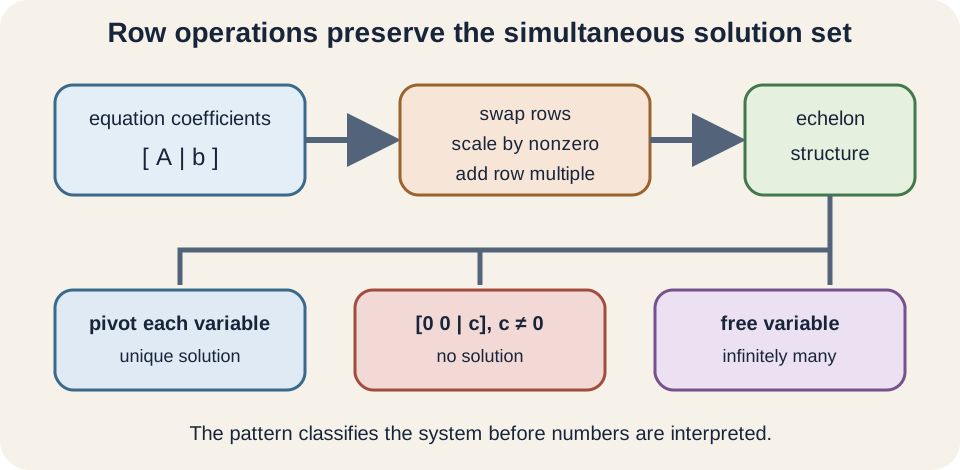
Three elementary row operations preserve the solution set. One may swap two rows, multiply a row by a nonzero constant, or replace one row with itself plus a multiple of another row. These operations mirror reordering equations, scaling an equation, and elimination. A zero multiplier cannot replace a row because it destroys information. Each operation should be recorded.

Row-echelon form makes back-substitution straightforward. Reduced row-echelon form isolates pivots and expresses dependent variables directly. A row such as $[0\ 0\mid3]$ means $0=3$ and signals inconsistency. A zero row $[0\ 0\mid0]$ signals a redundant equation. Matrix patterns encode the same solution classifications as graphs.

Worked row-reduction example

Represent $\begin{cases}x+2y=7\\3x-y=7\end{cases}$ as $\left[\begin{array}{cc|c}1&2&7\\3&-1&7\end{array}\right]$. Replace row two with row two minus three times row one. The new second row is $[0,-7\mid-14]$. Divide row two by negative seven to obtain $[0,1\mid2]$. Thus $y=2$.

Replace row one with row one minus two times row two. The first row becomes $[1,0\mid3]$. Reduced form is $\left[\begin{array}{cc|c}1&0&3\\0&1&2\end{array}\right]$. Thus $x=3$ and $y=2$. Pivot columns identify determined variables.

Substitute into the originals: $3+2(2)=7$ and $3(3)-2=7$. Both hold. Row operations preserve the exact solution set, so verification should agree. If it does not, an arithmetic error occurred. The original equations remain the authoritative check.

Modeling a ticket problem

A theater sells adult tickets for \12.00$and student tickets for$$8.00$. Suppose$250$tickets produce$$2600$in revenue. Let$a$be the number of adult tickets and$s$the number of student tickets. The count constraint is$a+s=250$. The revenue constraint is$12a+8s=2600$.

Multiply the count equation by negative eight and add it to the revenue equation. This gives $4a=600$, so $a=150$. Then $s=250-150=100$. Check revenue: $12(150)+8(100)=1800+800=2600$. Both counts are nonnegative integers, so the solution is contextually valid.

Units clarify the equations. In the first, tickets plus tickets gives tickets. In the second, dollars per adult ticket times adult tickets plus dollars per student ticket times student tickets gives dollars. The variables represent counts, not prices. Attaching units prevents coefficient confusion.

Modeling mixture and rate constraints

Suppose a chemist needs $10.0\,\mathrm L$ of a $30.0\%$ solution by mixing $20.0\%$ and $50.0\%$ solutions. Let $x$ and $y$ be volumes in liters. Total volume gives $x+y=10.0$. Solute amount gives $0.200x+0.500y=0.300(10.0)=3.00$. Percentages become decimal fractions before multiplication.

Substitute $x=10.0-y$. Then $0.200(10.0-y)+0.500y=3.00$. Simplifying gives $2.00+0.300y=3.00$, so $y=3.33\,\mathrm L$ and $x=6.67\,\mathrm L$. Weighted concentration lies between the two source concentrations. The volumes add to the target.

This model assumes volumes add directly and concentrations are expressed on a compatible basis. Real solution mixing can involve volume contraction or mass-based percentages. A chemistry problem must specify the concentration definition. Algebra solves the stated model, not every possible physical nuance. Assumptions belong with the answer.

More equations and unknowns

A system with three unknowns generally needs three independent linear constraints for a unique solution. Elimination can remove one variable from pairs of equations, producing a smaller two-variable system. Matrix row reduction organizes this process. Pivot count determines how many variables are constrained. Free variables parameterize families of solutions.

Having the same number of equations and unknowns does not guarantee uniqueness. Equations may be redundant or inconsistent. A square coefficient matrix has a unique solution only when it is invertible. Nonzero determinant provides that condition for square systems. Independence, not raw equation count, supplies information.

An overdetermined system has more equations than unknowns. It may still be consistent if all constraints intersect at one point, or inconsistent if measurements conflict. Data-fitting methods such as least squares then seek an approximate solution minimizing residuals. That next step replaces exact simultaneous satisfaction with optimal approximation. Exact systems provide the conceptual foundation.

Numerical sensitivity and rounding

Consider lines with nearly equal slopes. Their intersection may lie far away, and small coefficient changes can move it greatly. Rounded input data can therefore produce large output uncertainty. Exact-looking arithmetic does not guarantee an accurate physical estimate. Sensitivity is a property of the system structure.

Avoid rounding intermediate values unnecessarily. Keep fractions or guard digits through elimination and round only the final result to justified precision. Substitution verification can expose large residuals. In applied work, compare residual size with measurement uncertainty. A formally solved system may still be poorly determined.

Scaling equations can improve readability without changing solutions. Dividing a row by a large common factor reduces arithmetic size. Computational algorithms also pivot to avoid unstable divisions. These choices anticipate numerical linear algebra. Algebraic equivalence and numerical reliability are related but not identical.

Common misconceptions and repairs

One misconception reports an $x$ value without its paired $y$. A two-variable solution is an ordered pair. Back-substitute to determine the missing coordinate. Then test both originals. A coordinate alone does not identify an intersection.

Another misconception interprets $0=0$ as “all points work.” It means one transformed equation is redundant. Any remaining independent equation still constrains the solution. Parameterize the surviving line. The parameter must still satisfy that line’s relationship. In contrast, a false statement such as $0=3$ means no solution.

A third misconception changes only one side of an equation during elimination. Every operation must preserve equality. Multiply every term in a row, including the constant. Align variable columns and write absent terms with zero coefficients when useful. Structured bookkeeping prevents accidental model changes.

Practice with guided feedback

First, solve $\begin{cases}x+y=9\\2x-y=3\end{cases}$. Second, classify $\begin{cases}3x+6y=12\\x+2y=5\end{cases}$. Third, classify $\begin{cases}3x+6y=12\\x+2y=4\end{cases}$. Fourth, explain how each classification appears graphically. Verify every claim in the original equations.

Adding the first system equations gives $3x=12$, so $x=4$ and $y=5$. In the second system, multiplying the second equation by three gives $3x+6y=15$, contradicting the first constant twelve, so there is no solution. In the third system, multiplying the second by three reproduces the first, so infinitely many points on $x+2y=4$ solve it. Graphically these are intersecting, parallel, and coincident line pairs. Algebra and geometry agree.

For a matrix check, translate each system into an augmented matrix. Identify pivot columns and any contradiction row. For an application check, attach units and domain restrictions to variables. For a sensitivity check, compare line slopes. These habits make solving an evidence-backed classification process.

Retrieval and connection forward

Without looking back, define a system solution and the three possible solution counts. Solve one system by substitution and one by elimination. Explain what $0=0$ and $0=c$ for nonzero $c$ mean. Translate a system into an augmented matrix and name the three legal row operations. Finish by verifying an ordered pair in every original equation.

Matrices and row reduction will generalize these methods to larger systems. Linear transformations will explain determinants, pivots, rank, and null spaces structurally. Least squares will handle inconsistent data systems by minimizing residual error. Differential equations and circuits will produce coupled unknowns. The simultaneous-constraint idea remains unchanged.

Keep one organizing statement: a system solution satisfies every constraint at once. Graphs show shared intersections, substitution replaces equal expressions, elimination combines equalities to cancel variables, and row operations scale the same logic. Contradictions mean no solution, identities reveal dependence, and pivots identify determined variables. Contextual restrictions can narrow the algebraic solution set further. Verification completes the solution.