The Quadratic Formula Solves Every Quadratic Equation

Factoring can solve a quadratic equation quickly when its factors are recognizable, but not every quadratic factors conveniently over the integers or real numbers. Completing the square works systematically, and applying that process to a general quadratic produces one formula that covers every case. The quadratic formula solves $ax^2+bx+c=0$ whenever $a\ne0$. It returns exact real or complex roots and exposes the parabola’s symmetry through its algebraic structure. Understanding its derivation turns a memorized string into a reusable argument.

You will derive the formula through equivalence-preserving steps, interpret every symbol and grouping, classify roots using the discriminant, and connect root values to graph geometry. You will practice careful substitution with negative coefficients, simplify radicals, distinguish exact and approximate answers, and verify roots through substitution and Vieta’s relationships. You will also see why numerical implementations sometimes use an algebraically equivalent form to avoid cancellation error. Images will connect the derivation, discriminant, and geometry. The goal is to understand what the formula says before asking a calculator to evaluate it.

Begin a quadratic-equation problem by writing it in standard form with zero on one side. Identify $a$, $b$, and $c$ including their signs, and verify that $a\ne0$. Compute the discriminant separately before substituting the full formula. Preserve the entire numerator over the horizontal fraction bar and evaluate both branches of $\pm$. End by checking the roots against the original equation and the expected graph.

A quadratic equation must be in standard form

The standard quadratic equation is $ax^2+bx+c=0$, where $a$, $b$, and $c$ are constants and $a\ne0$. The coefficient $a$ multiplies the squared term, $b$ multiplies the linear term, and $c$ is the constant term. Some terms may be absent, which means their coefficients are zero. The equation must be rearranged before coefficient identification if its terms appear on both sides. Signs belong to the coefficients.

For $3x^2+7=5x$, subtract $5x$ from both sides to obtain $3x^2-5x+7=0$. Therefore $a=3$, $b=-5$, and $c=7$. Reading $b$ as positive five would change the equation. Parentheses around $-5$ during substitution protect the sign. Standard form is a data-extraction step.

The condition $a\ne0$ is structural. If $a=0$, the squared term disappears and the equation becomes linear or constant. The quadratic formula would then contain denominator $2a=0$, which is undefined. This failure is appropriate because a nonquadratic equation requires a different method. Checking $a$ prevents meaningless substitution.

Derivation begins by normalizing the squared coefficient

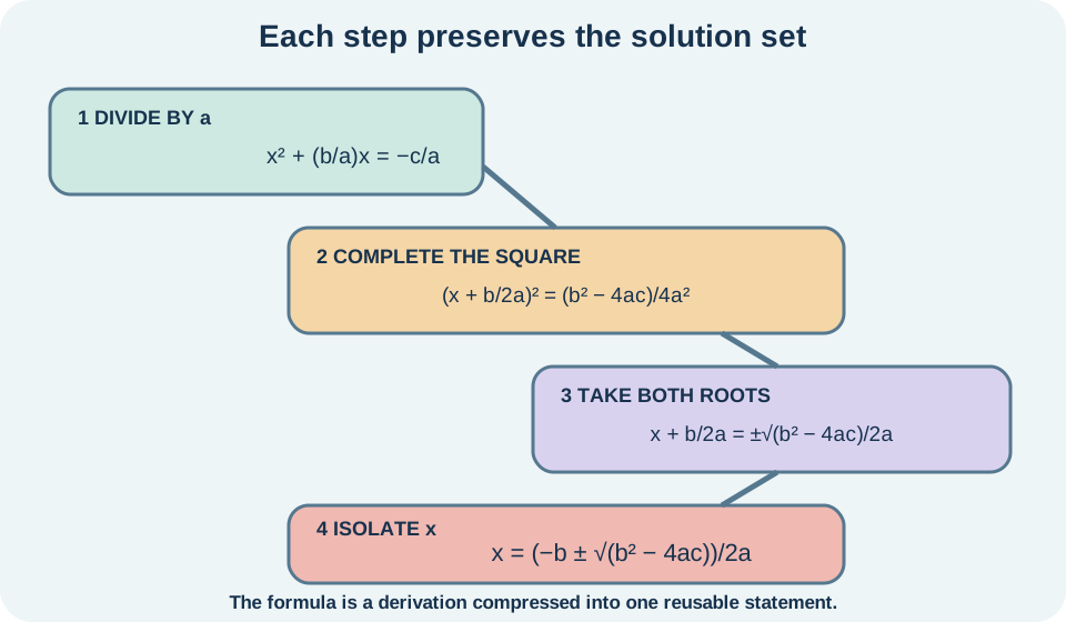
Start with $ax^2+bx+c=0$. Subtract $c$ from both sides to get $ax^2+bx=-c$. Divide every term by nonzero $a$, producing $x^2+\frac{b}{a}x=-\frac{c}{a}$. The horizontal fraction bars show division of the full coefficients. Dividing both sides by the same nonzero number preserves the solution set.

The purpose of this normalization is to make the coefficient of $x^2$ equal one. Completing the square uses half the linear coefficient inside the normalized expression. That coefficient is $\frac{b}{a}$, so half is $\frac{b}{2a}$. Squaring it gives $\frac{b^2}{4a^2}$. Add this same quantity to both sides to preserve equality.

The left side becomes a perfect square: $x^2+\frac{b}{a}x+\frac{b^2}{4a^2}=\left(x+\frac{b}{2a}\right)^2$. The right side becomes $-\frac{c}{a}+\frac{b^2}{4a^2}$. A common denominator $4a^2$ rewrites $-\frac{c}{a}$ as $-\frac{4ac}{4a^2}$. Therefore the right side is $\frac{b^2-4ac}{4a^2}$. Every term in the discriminant emerges from this common-denominator step.

Taking square roots creates two branches

After completing the square, the equation is $\left(x+\frac{b}{2a}\right)^2=\frac{b^2-4ac}{4a^2}$. If $u^2=v$, then $u=\pm\sqrt v$ when both square-root branches are considered. The radical symbol $\sqrt v$ conventionally denotes the principal square root, while $\pm$ restores the negative branch. Omitting $\pm$ would generally lose one solution. Squaring hides sign, so solving must recover it.

Taking roots gives $x+\frac{b}{2a}=\pm\frac{\sqrt{b^2-4ac}}{2a}$ under a consistent algebraic treatment, with branch signs absorbing denominator-sign conventions. Subtract $\frac{b}{2a}$ from both sides. The two terms now share denominator $2a$. Combining them yields $x=\frac{-b\pm\sqrt{b^2-4ac}}{2a}$. The entire numerator is divided by the entire denominator.

The formula is therefore completing the square in general symbols. It does not depend on guessing factors. Every algebraic step preserved equivalence for $a\ne0$, and both square-root branches were retained. This derivation explains why the method applies universally to quadratic equations. Memorization becomes easier when the structure is understood.

Read the formula as grouped operations

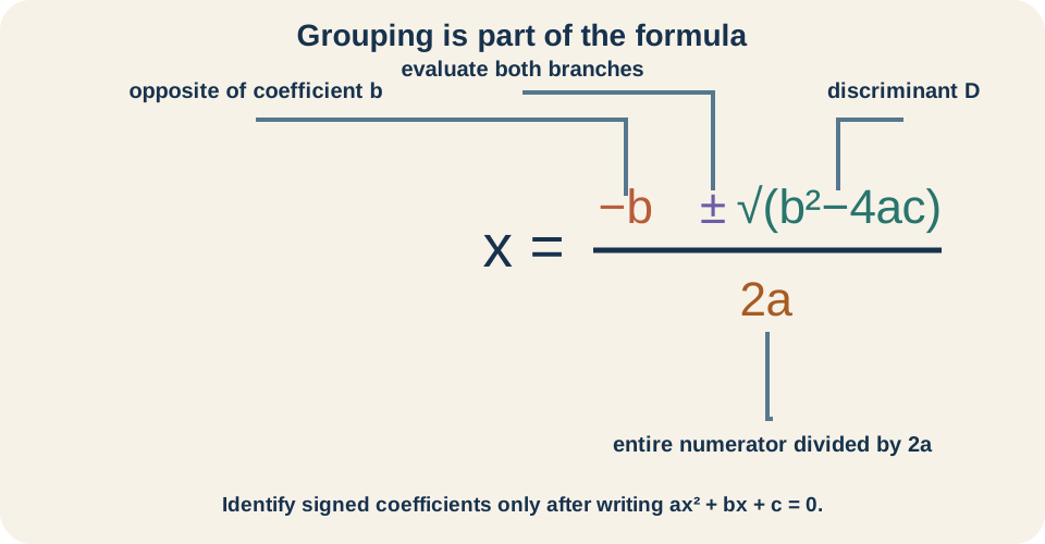
The formula is $x=\frac{-b\pm\sqrt{b^2-4ac}}{2a}$. The expression $-b$ means the additive opposite of coefficient $b$, not automatically a negative number. If $b=-5$, then $-b=-(-5)=5$. The symbol $\pm$ instructs two evaluations. The radical contains the full expression $b^2-4ac$.

The horizontal fraction bar groups the complete numerator and denominator. Both $-b$ and the radical are divided by $2a$. Writing $-b\pm\sqrt{\frac{b^2-4ac}{2a}}$ changes the expression because only the radical would be divided. Writing $\frac{-b\pm\sqrt{b^2-4ac}}{2}a$ can also be read as multiplication by $a$ after division by two. Parentheses and a full fraction bar protect intended structure.

Order of operations matters inside the discriminant. Compute $b^2$, compute the product $4ac$ with coefficient signs, then subtract that product. If $c$ is negative, $4ac$ is negative and subtracting it becomes addition. Work the discriminant on a separate line. This reduces sign and grouping errors.

The discriminant classifies the solution type

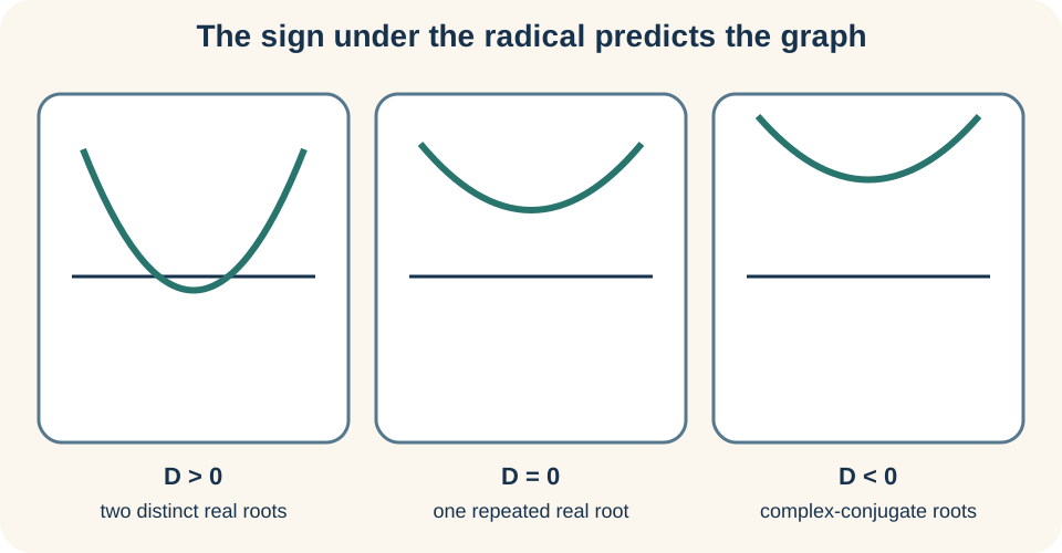
The discriminant is $D=b^2-4ac$. It is called a discriminant because its sign distinguishes root cases. If $D>0$, the radical is a positive real number and the two $\pm$ branches yield distinct real roots. If $D=0$, the radical is zero and both branches collapse to the same real root. If $D<0$, the roots are complex and the graph has no real horizontal intercepts.

For $3x^2+2x+5=0$, $D=2^2-4(3)(5)=4-60=-56$. The negative result predicts two complex-conjugate roots. No real input makes the quadratic output zero. Because $a=3>0$, its parabola opens upward and remains above the horizontal axis. The discriminant supplies this geometric information without fully solving.

For $x^2-6x+9=0$, $D=(-6)^2-4(1)(9)=36-36=0$. The repeated root is $x=\frac{6}{2}=3$. The quadratic factors as $(x-3)^2$, so the graph touches the horizontal axis at its vertex. Algebra and geometry tell the same story. A repeated root has multiplicity two.

Solve a factorable example and cross-check it

Solve $2x^2-3x-2=0$. The coefficients are $a=2$, $b=-3$, and $c=-2$. The discriminant is $D=(-3)^2-4(2)(-2)=9+16=25$. Its principal square root is five. Substitution gives $x=\frac{3\pm5}{4}$.

The positive branch gives $x=\frac{3+5}{4}=2$. The negative branch gives $x=\frac{3-5}{4}=-\frac{1}{2}$. Both answers are exact. The two values should be reported as a solution set rather than combined. The $\pm$ operation has now been fully evaluated.

Factoring independently gives $(2x+1)(x-2)=0$, which yields the same roots. Substitution of $x=2$ gives $8-6-2=0$. Substitution of $x=-\frac{1}{2}$ gives $2\left(\frac{1}{4}\right)+\frac{3}{2}-2=0$. Agreement among formula, factors, and substitution is strong verification. Vieta’s sum and product provide two additional coefficient-level checks.

Irrational roots can remain exact

Solve $x^2-2x-1=0$. Here $a=1$, $b=-2$, and $c=-1$, so $D=4+4=8$. The formula gives $x=\frac{2\pm\sqrt8}{2}$. Simplify $\sqrt8=\sqrt{4\cdot2}=2\sqrt2$. Therefore the exact roots are $x=1\pm\sqrt2$.

An exact radical preserves complete mathematical information. Decimal approximations are $1+\sqrt2\approx2.414$ and $1-\sqrt2\approx-0.414$. Use the approximation symbol $\approx$ rather than the equality symbol when digits are rounded. The required precision should come from the problem context. Intermediate rounding can degrade a later calculation.

The root midpoint is one, which matches $-\frac{b}{2a}=1$. Their equal displacement from one is $\sqrt2$. This symmetry check is visible directly in $1\pm\sqrt2$. The corresponding vertex axis is $x=1$. Exact form exposes structure that decimals can hide.

Complex roots extend the number system

When $D<0$, write $\sqrt{-m}=i\sqrt m$ for positive $m$, where $i^2=-1$. For $x^2+4x+13=0$, the discriminant is $16-52=-36$. The formula gives $x=\frac{-4\pm\sqrt{-36}}{2}=\frac{-4\pm6i}{2}$. Simplifying gives $x=-2\pm3i$. The roots form a complex-conjugate pair.

Real-coefficient quadratics produce nonreal roots in conjugate pairs. If $p+qi$ is a root, then $p-qi$ is also a root. Their imaginary parts cancel in the sum and their product is real. This pairing keeps the polynomial coefficients real. The graph over real inputs still has no horizontal-axis intersections.

Complex roots are genuine solutions because substitution into the polynomial gives zero under complex arithmetic. They should not be reported as “no solution” unless the requested domain is explicitly real numbers. The statement “no real solutions” is precise. Expanding the number system preserves algebraic closure. Domain language determines the appropriate conclusion.

The formula encodes the axis of symmetry

Write the two roots as $r_1=\frac{-b+\sqrt D}{2a}$ and $r_2=\frac{-b-\sqrt D}{2a}$. Their average is $\frac{r_1+r_2}{2}=-\frac{b}{2a}$ because the radical terms cancel. This value is exactly the axis of symmetry of $y=ax^2+bx+c$. The two roots, when real, lie symmetrically around that axis. The formula contains graph geometry.

Their difference is $r_1-r_2=\frac{\sqrt D}{a}$ under the chosen ordering. The absolute separation is $\frac{\sqrt D}{|a|}$ for $D\ge0$. Larger positive discriminant generally spreads real roots farther apart relative to leading scale. When $D=0$, separation is zero. The repeated root lies on the axis.

The vertex vertical coordinate also relates to the discriminant. Completing the square gives vertex height $-\frac{D}{4a}$. For an upward-opening parabola, a positive discriminant makes this height negative, leading to two crossings. A zero discriminant places the vertex on the axis. A negative discriminant makes the height positive, producing no real crossing.

Vieta’s relationships provide fast checks

For roots $r_1$ and $r_2$, the factored form is $a(x-r_1)(x-r_2)$. Expanding gives $ax^2-a(r_1+r_2)x+ar_1r_2$. Comparing with $ax^2+bx+c$ gives $r_1+r_2=-\frac{b}{a}$ and $r_1r_2=\frac{c}{a}$. These are Vieta’s relationships for a quadratic. They follow from coefficient comparison.

For $2x^2-3x-2=0$, roots $2$ and $-\frac{1}{2}$ sum to $\frac{3}{2}$. The coefficient relation gives $-\frac{-3}{2}=\frac{3}{2}$. Their product is $-1$, matching $\frac{-2}{2}=-1$. Both checks pass. A sign error in one root would likely fail at least one relation.

Vieta’s relationships can sometimes answer questions without solving. If a problem asks only for the sum of roots, $-\frac{b}{a}$ is immediate. If it asks for the product, use $\frac{c}{a}$. These formulas include multiplicity and complex roots. They are structural consequences, not separate coincidences.

Choose among factoring, square completion, and the formula

Factoring is often fastest when integer or simple rational factors are visible. Completing the square is especially useful for vertex form and derivation. The quadratic formula is systematic and works regardless of convenient factorization. Graphing estimates real roots and reveals geometry. No method is universally best for every goal.

For $x^2-9=0$, difference-of-squares factoring gives $(x-3)(x+3)=0$ immediately. The formula works but adds unnecessary arithmetic. For $x^2+6x+5=0$, factoring is also straightforward. For $3x^2+2x+5=0$, the formula naturally reveals complex roots. Method choice should respond to structure.

An exact symbolic answer may be preferable even when software can approximate instantly. Factored form may reveal multiplicity, vertex form may reveal extrema, and formula form may reveal coefficient dependence. Converting among representations validates results. Tool use should support interpretation rather than replace it. The best representation depends on the question being answered.

Applications require interpreting roots in context

Suppose projectile height is modeled by $h(t)=-4.9t^2+18t+1.2$, with height in meters and time in seconds. Setting $h(t)=0$ asks when the model reaches ground level. The quadratic formula can produce one positive and one negative time. The positive root may represent impact after launch. The negative root can be algebraically valid but outside the modeled time domain $t\ge0$.

Units belong to coefficients. The $t^2$ coefficient has units $\frac{\mathrm m}{\mathrm{s^2}}$, the linear coefficient has $\frac{\mathrm m}{\mathrm s}$, and the constant has meters. Every term therefore has height units. The formula’s root has seconds after dimensional cancellation. A numerical answer without time units is incomplete in the application.

Not every root represents a physically possible state. Lengths may need to be positive, counts may need to be nonnegative integers, and model validity may cover only a finite interval. Rejecting an inadmissible root does not make it algebraically false. It makes it irrelevant to the chosen context. State the restriction explicitly.

Numerical computation can suffer cancellation

The standard formula is algebraically correct, but finite-precision computation can lose accuracy when $-b$ and $\sqrt D$ are nearly equal and opposite. Their subtraction can cancel leading digits, leaving a small result contaminated by rounding. This issue matters for very different root magnitudes. Hand calculations at classroom scale may not reveal it. Numerical analysis distinguishes symbolic correctness from stable evaluation.

One stable strategy computes the branch with addition of same-sign magnitudes and then uses the root product $r_1r_2=\frac{c}{a}$ to obtain the other root. An equivalent implementation may define $q=-\frac{1}{2}\left(b+\operatorname{sgn}(b)\sqrt D\right)$, then use roots $\frac{q}{a}$ and $\frac{c}{q}$ when appropriate. The sign function selects the sign of $b$. This avoids subtracting nearly equal large quantities. Exceptional cases such as $q=0$ require separate handling in software.

This refinement does not change the mathematics of the roots. It changes how floating-point arithmetic reaches them. Software libraries may use such rearrangements internally. The lesson is broader than quadratics: equivalent formulas can have different numerical stability. Verification and scale awareness remain important even with exact algebra behind the computation.

Common errors and corrective habits

The most common error misidentifies coefficient signs. Write $a$, $b$, and $c$ on a separate line after moving all terms to one side. Enclose negative values in parentheses during substitution. Another error squares $b$ incorrectly, especially when $b<0$. Remember $(-b_0)^2$ is positive.

A grouping error places only the radical over $2a$. Write the formula with a full horizontal fraction and copy the numerator as one grouped expression. Another error evaluates only the plus branch. Separate the work into $x_+$ and $x_-$ lines. If $D=0$, explain why the two branches coincide.

A reporting error rounds too early or says “no solution” for a negative discriminant without naming the real-number domain. Keep radicals exact until approximation is requested. Simplify square factors from radicals. Verify with substitution, Vieta’s sum and product, discriminant type, and graph geometry. Multiple independent checks turn a procedural answer into a reliable result.

A complete worked synthesis

Solve $3x^2+4x-2=0$. Coefficients are $a=3$, $b=4$, and $c=-2$. The discriminant is $D=4^2-4(3)(-2)=16+24=40>0$, so two distinct real roots are expected. The formula gives $x=\frac{-4\pm\sqrt{40}}{6}$. Simplifying $\sqrt{40}=2\sqrt{10}$ yields $x=\frac{-2\pm\sqrt{10}}{3}$.

The approximate roots are $0.387$ and $-1.721$ to three decimals. Their average is approximately $-0.667$, matching $-\frac{b}{2a}=-\frac{4}{6}$. Their sum is $-\frac{4}{3}$ and product is $-\frac{2}{3}$ in exact form, matching Vieta’s relations. One root is positive and one negative because their product is negative. The graph must cross once on each side of zero.

Substitution can be done exactly or numerically. Exact substitution is algebraically conclusive but can be lengthy with radicals. Numerical substitution should return values close to zero, with residual size reflecting rounding. Factoring over radicals using the two roots would reconstruct the polynomial. The agreement among methods supports the solution.

Retrieval and connection forward

Without looking back, derive the quadratic formula in outline by normalizing, completing the square, taking both square-root branches, and isolating $x$. Explain why $a\ne0$, why $\pm$ is necessary, and why the entire numerator lies over $2a$. Define the discriminant and connect its sign to graph intersections. Then state Vieta’s sum and product checks. If a symbol cannot be explained, return to the derivation step that created it.

The formula supports quadratic-function analysis, polynomial factorization, complex numbers, conic sections, and applied modeling. Completing the square connects it to vertex geometry. Vieta’s relationships extend to higher-degree polynomials. Numerical stability introduces computational mathematics. In calculus and physics, roots identify events such as crossings, turning constraints, and feasible times.

The enduring insight is that a universal method can still reveal structure. The formula is not a black box; it is completed-square algebra compressed into one line. Its discriminant classifies solutions, its center gives the axis of symmetry, and its branches recover paired roots. Exact forms preserve relationships while approximations serve measurement and computation. Understanding these layers makes the quadratic formula a theorem you can use intelligently rather than a chant you must remember.