The Formal Definition of a Limit

Learning objectives

By the end of this lesson, you should be able to:

• state the epsilon-delta definition of a finite limit;
• explain the roles of $\varepsilon$ and $\delta$;
• interpret the quantifiers “for every” and “there exists”;
• translate the absolute-value inequalities in the definition into intervals;
• explain why the condition $0<|x-a|$ excludes the value $x=a$;
• determine a suitable $\delta$ for a given $\varepsilon$;
• distinguish the process of discovering a proof from the presentation of the proof; and
• construct epsilon-delta proofs for elementary limits.

We developed the idea of a limit using tables, graphs, and formulas in the first lesson on limits. In the previous lesson, we made the direction of approach explicit and used one-sided limits to determine whether a two-sided limit exists.

Those ideas are useful, but phrases such as “approaches,” “gets closer to,” and “trends toward” are descriptions, not definitions.

We are now ready to replace that informal language with the formal mathematical definition of a limit.

The formal definition

In symbols,

$$\boxed{ \forall\varepsilon>0,\ \exists\delta>0 \text{ such that } 0<|x-a|<\delta \Longrightarrow |f(x)-L|<\varepsilon. }$$

Every part of this statement matters.

Understanding epsilon

The quantity

$$|f(x)-L|$$

measures the distance between the output $f(x)$ and the proposed limiting value $L$.

Therefore, $|f(x)-L|<\varepsilon$

means that $f(x)$ must lie within a distance $\varepsilon$ of $L$.

Equivalently,

$$L-\varepsilon<f(x)<L+\varepsilon.$$

The number $\varepsilon$ specifies the required output tolerance.

The definition begins with

$$\forall\varepsilon>0.$$

That means the requirement must work for every positive tolerance, no matter how small.

We do not get to choose a convenient $\varepsilon$. The definition requires us to respond successfully to any positive $\varepsilon$ that is given.

Understanding delta

The quantity

$$|x-a|$$

measures the distance between the input $x$ and the target input $a$.

Thus, $|x-a|<\delta$

means

$$a-\delta<x<a+\delta.$$

The number $\delta$ specifies an input tolerance around $a$.

The purpose of an epsilon-delta proof is to show that, for any requested output tolerance $\varepsilon$, we can choose an input tolerance $\delta$ that guarantees the desired output condition.

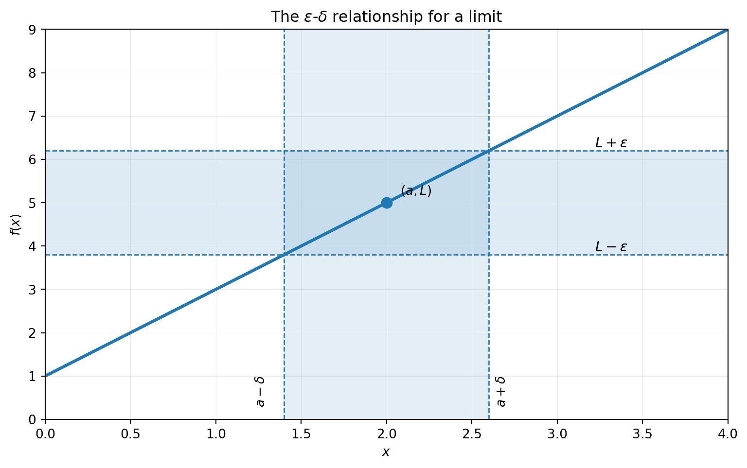
The figure below shows this relationship. The vertical region represents inputs within $\delta$ of $a$, while the horizontal band represents outputs within $\varepsilon$ of $L$.

The mathematical claim is that we can make the output band as narrow as we wish and still find a sufficiently narrow input interval that keeps the function inside it.

Why the target point is excluded

The definition does not say merely

$$|x-a|<\delta.$$

It says

$$0<|x-a|<\delta.$$

The inequality

$$0<|x-a|$$

means

$$x\neq a.$$

This exclusion is deliberate. A limit describes the trend of a function near $a$; it does not require the function to have any particular value at $a$ itself.

This is why a limit may exist even when $f(a)$ is undefined, as we saw with removable discontinuities in the first lesson on limits.

The order of the quantifiers matters

The formal definition says

$$\forall\varepsilon>0,\ \exists\delta>0.$$

In words:

For every positive $\varepsilon$, there exists a positive $\delta$ that works.

The choice of $\delta$ may depend on $\varepsilon$.

That is not what the definition requires.

A useful way to think about the logical order is:

1. An output tolerance $\varepsilon>0$ is specified.

2. We choose a suitable input tolerance $\delta>0$.

3. We assume an input satisfies

   $$0<|x-a|<\delta.$$

4. We prove that this guarantees

   $$|f(x)-L|<\varepsilon.$$

The proof must work for an arbitrary positive $\varepsilon$.

First proof: a linear function

Prove that

$$\boxed{ \lim_{x\to2}(3x+1)=7. }$$

Discovering the input tolerance

We want to guarantee

$$|(3x+1)-7|<\varepsilon.$$

Simplify the left side:

$$\begin{aligned} |(3x+1)-7| &= |3x-6| \\ &= |3(x-2)| \\ &= 3|x-2|. \end{aligned}$$

Therefore, it is sufficient to require

$$3|x-2|<\varepsilon.$$

Dividing by $3$ gives

$$|x-2|<\frac{\varepsilon}{3}.$$

This suggests the choice

$$\boxed{ \delta=\frac{\varepsilon}{3}. }$$

That backward work discovers the value of $\delta$. It is not yet the formal proof.

Presenting the proof

Let $\varepsilon>0$ be arbitrary.

Choose

$$\delta=\frac{\varepsilon}{3}.$$

Suppose

$$0<|x-2|<\delta.$$

Then

$$\begin{aligned} |(3x+1)-7| &= 3|x-2| \\ &< 3\delta \\ &= 3\left(\frac{\varepsilon}{3}\right) \\ &= \varepsilon. \end{aligned}$$

Therefore,

$$0<|x-2|<\delta \Longrightarrow |(3x+1)-7|<\varepsilon.$$

Since this works for every $\varepsilon>0$, the formal definition gives

$$\boxed{ \lim_{x\to2}(3x+1)=7. }$$

A general linear limit

The same reasoning proves a stronger result.

Suppose

$$f(x)=mx+b.$$

We claim

$$\boxed{ \lim_{x\to a}(mx+b)=ma+b. }$$

For $m\neq0$,

$$\begin{aligned} |(mx+b)-(ma+b)| &= |mx-ma| \\ &= |m(x-a)| \\ &= |m||x-a|. \end{aligned}$$

To make this less than $\varepsilon$, it is sufficient to require

$$|x-a|<\frac{\varepsilon}{|m|}.$$

So choose

$$\delta=\frac{\varepsilon}{|m|}.$$

Then $0<|x-a|<\delta$

implies

$$\begin{aligned} |(mx+b)-(ma+b)| &= |m||x-a| \\ &< |m|\delta \\ &= |m|\frac{\varepsilon}{|m|} \\ &= \varepsilon. \end{aligned}$$

Therefore,

$$\boxed{ \lim_{x\to a}(mx+b)=ma+b. }$$

If $m=0$, the function is constant and the result follows immediately.

This proof establishes an entire family of limits rather than calculating only one example.

A more difficult proof: a quadratic function

Linear functions are unusually convenient because

$$|f(x)-L|$$

reduces directly to a constant multiple of $|x-a|$.

For nonlinear functions, another bound may be necessary.

We want to prove

$$\boxed{ \lim_{x\to2}x^2=4. }$$

Begin with the required output condition:

$$|x^2-4|<\varepsilon.$$

Factor:

$$|x^2-4| = |x-2||x+2|.$$

We can control $|x-2|$ using $\delta$, but $|x+2|$ also depends on $x$.

We therefore need to bound $|x+2|$.

A convenient way to do this is to restrict $x$ to a fixed neighborhood around $2$. We choose the simple condition $|x-2|<1$. The number $1$ is not mathematically special; any sufficiently small fixed positive bound could be used. Choosing $1$ is convenient because it immediately places $x$ between two simple values and gives an easy numerical bound for $|x+2|$.

Suppose, then, that $|x-2|<1$. We obtain

$$\begin{aligned} |x-2| &< 1,\\ -1 &< x-2 < 1,\\ 1 &< x < 3,\\ 3 &< x+2 < 5. \end{aligned}$$

Thus $|x+2|<5$. Therefore, under the restriction $|x-2|<1$,

$$\begin{aligned} |x^2-4| &=|x-2||x+2|\\ &<5|x-2|. \end{aligned}$$

This bound is local: it has been established for inputs satisfying $|x-2|<1$. Under that restriction, to guarantee that $|x^2-4|<\varepsilon$, it is sufficient to require $|x-2|<\frac{\varepsilon}{5}$. We therefore need both $|x-2|<1$ and $|x-2|<\frac{\varepsilon}{5}$, so choose

$$\boxed{ \delta=\min\left(1,\frac{\varepsilon}{5}\right). }$$

Formal proof

Let $\varepsilon>0$ be arbitrary. Choose

$$\delta=\min\left(1,\frac{\varepsilon}{5}\right).$$

Suppose

$$0<|x-2|<\delta.$$

Because $\delta\le1$, we have

$$|x-2|<1,$$

which implies

$$1<x<3,$$

and therefore

$$|x+2|<5.$$

Also, because $\delta\le\frac{\varepsilon}{5}$, we have

$$|x-2|<\frac{\varepsilon}{5}.$$

Because $|x-2|<1$ established the local bound $|x+2|<5$, we may now write

$$\begin{aligned} |x^2-4| &= |x-2||x+2| \\ &< 5|x-2| \\ &< 5\left(\frac{\varepsilon}{5}\right) \\ &= \varepsilon. \end{aligned}$$

Therefore,

$$0<|x-2|<\delta \Longrightarrow |x^2-4|<\varepsilon.$$

By the formal definition,

$$\boxed{ \lim_{x\to2}x^2=4. }$$

Choosing between multiple bounds

The previous proof required two restrictions. The condition

$$|x-2|<1$$

restricts $x$ to a neighborhood in which $|x+2|<5$. Consequently, the estimate $|x^2-4|<5|x-2|$ is valid within that neighborhood; it is not being asserted as a global inequality. Once this local bound is established, the condition

$$|x-2|<\frac{\varepsilon}{5}$$

is sufficient to guarantee

$$|x^2-4|<\varepsilon,$$

which places the function value within the specified output tolerance around the limit.

Choosing

$$\delta=\min\left(1,\frac{\varepsilon}{5}\right)$$

guarantees both restrictions simultaneously.

This pattern occurs frequently in epsilon-delta proofs. One bound controls an inconvenient part of the expression, while another ensures that the function remains within the required $\varepsilon$-tolerance of the limit.

Proof development versus proof presentation

When constructing an epsilon-delta proof, it is often useful to begin with the desired inequality and work backward during scratch work to determine a suitable value of $\delta$.

During development, begin with the desired result:

$$|f(x)-L|<\varepsilon$$

and manipulate it until you determine what restriction on $|x-a|$ would guarantee it.

That process suggests a suitable $\delta$.

Once a suitable $\delta$ has been identified, the formal proof verifies that the choice satisfies the definition:

1. Let $\varepsilon>0$.

2. Choose the $\delta$ discovered during the preliminary work.

3. Assume

   $$0<|x-a|<\delta.$$

4. Use that assumption to prove

   $$|f(x)-L|<\varepsilon.$$

5. Conclude that the limit follows from the formal definition.

Test Your Knowledge

For each proof problem, first perform enough scratch work to determine a suitable $\delta$. Then write a complete formal proof using the epsilon-delta definition.

1. Interpret the definition

Suppose

$$\lim_{x\to3}f(x)=8.$$

Explain in words what the statement

$$\varepsilon=0.1$$

requires the formal definition to guarantee.

Solution

The output must satisfy

$$|f(x)-8|<0.1.$$

Equivalently,

$$7.9<f(x)<8.1.$$

The formal definition guarantees that there is some $\delta>0$ such that every domain value satisfying

$$0<|x-3|<\delta$$

also satisfies

$$7.9<f(x)<8.1.$$

2. Find an input tolerance for a specified output tolerance

For $f(x)=3x+1$ and $\lim_{x\to2}f(x)=7$, find a suitable $\delta$ when $\varepsilon=0.06$.

Solution

We found earlier that

$$\delta=\frac{\varepsilon}{3}$$

works.

Therefore, $\delta=\frac{0.06}{3}=0.02.$

If

$$0<|x-2|<0.02,$$

then

$$\begin{aligned} |(3x+1)-7| &=3|x-2|\\ &<3(0.02)\\ &=0.06. \end{aligned}$$

Thus, $\boxed{\delta=0.02}$ is a suitable choice.

3. Prove a linear limit

Use the formal definition to prove

$$\lim_{x\to4}(2x-3)=5.$$

Solution

Let $\varepsilon>0$.

We want

$$|(2x-3)-5|<\varepsilon.$$

Since

$$|(2x-3)-5| = |2x-8| = 2|x-4|,$$

choose

$$\delta=\frac{\varepsilon}{2}.$$

Suppose

$$0<|x-4|<\delta.$$

Then

$$\begin{aligned} |(2x-3)-5| &= 2|x-4| \\ &< 2\delta \\ &= 2\left(\frac{\varepsilon}{2}\right) \\ &= \varepsilon. \end{aligned}$$

Therefore, by the formal definition,

$$\boxed{ \lim_{x\to4}(2x-3)=5. }$$

4. Determine whether a proposed input tolerance works

A student wants to prove

$$\lim_{x\to1}(5x+2)=7$$

and chooses

$$\delta=\varepsilon.$$

Does this choice guarantee the epsilon condition for every $\varepsilon>0$?

Solution

No.

We have

$$|(5x+2)-7| = 5|x-1|.$$

If we know only that

$$|x-1|<\varepsilon,$$

then we can conclude only that

$$|(5x+2)-7|<5\varepsilon,$$

not that it is less than $\varepsilon$.

A suitable choice is

$$\boxed{ \delta=\frac{\varepsilon}{5}. }$$

Then $|x-1|<\delta$

guarantees

$$|(5x+2)-7| < 5\frac{\varepsilon}{5} = \varepsilon.$$

5. Construct a quadratic proof

Use the formal definition to prove

$$\lim_{x\to1}x^2=1.$$

Solution

We need to control

$$|x^2-1| = |x-1||x+1|.$$

We need a fixed bound on $|x+1|$. Choose the convenient restriction $|x-1|<1$. The choice of $1$ is not unique; it is used because it gives simple bounds on $x$ and therefore on $|x+1|$.

From $|x-1|<1$, we have $0<x<2$, so $1<x+1<3$ and therefore $|x+1|<3$.

Thus, under the restriction $|x-1|<1$,

$$|x^2-1| < 3|x-1|.$$

Choose

$$\delta=\min\left(1,\frac{\varepsilon}{3}\right).$$

Now suppose

$$0<|x-1|<\delta.$$

Because $\delta\le1$, we have $|x-1|<1$, so the local bound $|x+1|<3$ applies. Because $\delta\le\frac{\varepsilon}{3}$, we also have $|x-1|<\frac{\varepsilon}{3}$. Therefore,

$$\begin{aligned} |x^2-1| &= |x-1||x+1| \\ &< 3|x-1| \\ &< 3\left(\frac{\varepsilon}{3}\right) \\ &= \varepsilon. \end{aligned}$$

Hence,

$$\boxed{ \lim_{x\to1}x^2=1. }$$

6. Find the flaw in a proof

A student claims to have proved

$$\lim_{x\to2}x^2=4$$

as follows:

Let $\varepsilon>0$. Choose $\delta=\varepsilon$. If $0<|x-2|<\delta$, then

$$|x^2-4|=|x-2||x+2|<\varepsilon.$$

Therefore the limit is $4$.

Identify the error.

Solution

The student correctly factors

$$|x^2-4| = |x-2||x+2|,$$

but controls only the factor $|x-2|$.

From

$$|x-2|<\varepsilon$$

we cannot conclude

$$|x-2||x+2|<\varepsilon$$

unless we also control $|x+2|$.

For example, requiring

$$|x-2|<1$$

gives

$$|x+2|<5.$$

We can then choose

$$\delta=\min\left(1,\frac{\varepsilon}{5}\right),$$

which controls both factors sufficiently to complete the proof.

7. Build the proof yourself

Use the formal definition to prove

$$\lim_{x\to3}x^2=9.$$

Determine a suitable $\delta$ and write a complete epsilon-delta proof.

Solution

We begin with

$$|x^2-9| = |x-3||x+3|.$$

We first need a fixed bound on $|x+3|$. Choose the convenient restriction $|x-3|<1$. Again, the value $1$ is not required; it is a simple choice that gives useful bounds on $x$.

From $|x-3|<1$, we have $2<x<4$, so $5<x+3<7$ and therefore $|x+3|<7$.

Thus, under the restriction $|x-3|<1$,

$$|x^2-9| = |x-3||x+3| < 7|x-3|.$$

Under this restriction, to guarantee

$$|x^2-9|<\varepsilon,$$

it is sufficient to require

$$|x-3|<\frac{\varepsilon}{7}.$$

Choose

$$\delta=\min\left(1,\frac{\varepsilon}{7}\right).$$

Let $\varepsilon>0$ and suppose

$$0<|x-3|<\delta.$$

Because $\delta\le1$, we have $|x-3|<1$, so the local bound $|x+3|<7$ applies. Because $\delta\le\frac{\varepsilon}{7}$, we also have $|x-3|<\frac{\varepsilon}{7}$. Therefore,

$$\begin{aligned} |x^2-9| &= |x-3||x+3| \\ &< 7|x-3| \\ &< 7\left(\frac{\varepsilon}{7}\right) \\ &= \varepsilon. \end{aligned}$$

Therefore,

$$\boxed{ \lim_{x\to3}x^2=9. }$$