Continuity Makes Local Behavior Trustworthy

Continuity says that nearby inputs produce outputs that align with the value assigned at the point. That statement sounds visually simple, yet it supports some of calculus’s most important existence and approximation arguments. Continuity lets mathematicians move limits through familiar functions, guarantee intermediate outputs, and control local error. It is also a modeling assumption that can succeed or fail depending on the scale of observation. This article develops continuity as a form of mathematical trust with explicit conditions.

Move beyond the unbroken-pencil metaphor

The familiar instruction to draw a graph without lifting a pencil captures part of continuity’s visual intuition. It suggests the absence of holes, jumps, and vertical breaks. However, drawing speed, graph resolution, and domain endpoints make the metaphor unreliable as a definition. A graph can hide a missing point. A function can also be continuous on a disconnected domain relative to that domain.

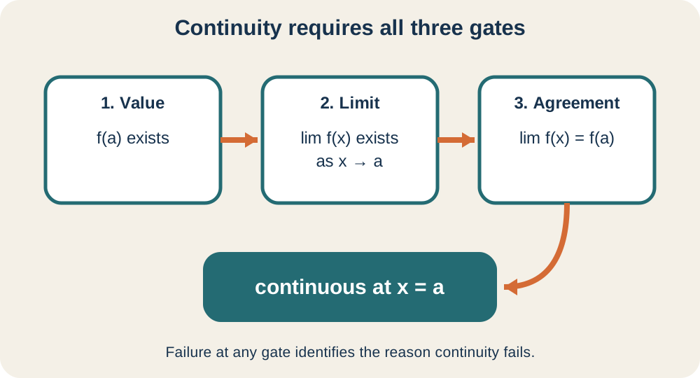
Limits provide the precise replacement. Continuity at $x=a$ requires $f(a)$ to exist, $\lim_{x\to a}f(x)$ to exist, and those quantities to be equal. The point value and nearby target are logically distinct. Their agreement creates continuity. Naming each condition reveals exactly why a function fails.

This definition makes continuity local. A function can be continuous at one point and discontinuous at another. It can be continuous throughout an interval while behaving very differently elsewhere. A local conclusion should not be promoted to a global one without checking the entire relevant domain. The interval under discussion belongs in every theorem claim.

Interpret continuity as stable input-output behavior

Continuity means that sufficiently small input changes produce arbitrarily small output changes near the chosen point. The statement does not require a small slope. A steep line is continuous even though its output changes rapidly. It requires control rather than flatness. The input tolerance may need to be very small when sensitivity is high.

The epsilon-delta definition makes this control exact. For every $\varepsilon>0$, there must be a $\delta>0$ such that $|x-a|<\delta$ implies $|f(x)-f(a)|<\varepsilon$. Epsilon is an allowed output error. Delta is a sufficient input tolerance. The order matters because the output demand is set before the input response is chosen.

This language supports measurement and computation. If an instrument’s input uncertainty is bounded, continuity helps bound the resulting output variation locally. The needed delta can depend on the point and the desired epsilon. Continuity alone does not guarantee one uniform tolerance across an entire unbounded domain. Stronger uniform-continuity conditions address that global requirement.

Separate nearby behavior from assigned value

Changing one function value does not change a limit. Suppose $f(x)=x^2$ for $x\ne2$ but $f(2)=100$. Nearby outputs still approach four. The function value is one hundred. The mismatch creates a removable discontinuity.

This example shows why substitution is not the definition of a limit. The limit ignores the value at the approached point and studies punctured neighborhoods. Continuity adds the value back into the comparison. When a known continuous function is used, substitution becomes justified by a theorem. It should not be used circularly to prove the continuity it assumes.

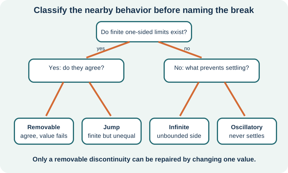
Only a removable discontinuity can be repaired by redefining one point. If left and right neighborhoods approach different targets, no assigned value can reconcile them. If values become unbounded or oscillate without settling, a single point also has no influence. The repair test therefore doubles as a classification tool. It asks whether the failure lives at the point or throughout nearby behavior.

Treat continuity relative to domain

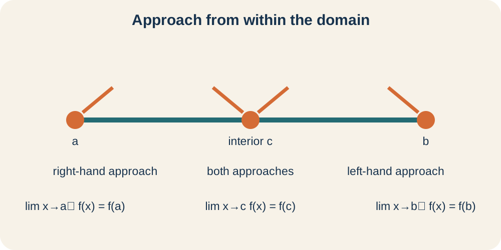
Approach uses inputs belonging to the function’s domain. At an interior point, values can approach from both sides. At a left endpoint, only right-side inputs may exist. At a right endpoint, only left-side inputs may exist. Continuity uses the approaches available within the domain.

The square-root function is continuous at zero on $[0,\infty)$. Its right-hand limit equals zero, which matches its value. There is no requirement for real inputs approaching zero from the left because the function has no such domain points. This is not an exception to continuity. It is the definition applied relative to the domain.

Closed-interval theorems encode these endpoint conventions. Continuity on $[a,b]$ means two-sided continuity inside, right continuity at $a$, and left continuity at $b$. Every point of the interval is covered. A missing interior point can invalidate the theorem even if the endpoints behave well. Domain language prevents hidden gaps in the hypotheses.

Build continuity from known components

Polynomials are continuous for all real inputs. Rational functions are continuous wherever their denominators are nonzero. Exponential, logarithmic, radical, and trigonometric functions are continuous on their natural domains. These foundational results let larger models inherit continuity. Domain restrictions remain part of the inheritance.

Sums, differences, products, and constant multiples of continuous functions are continuous where their components are defined. Quotients require a nonzero denominator. Compositions require the inner function to be continuous at the input and the outer function to be continuous at the resulting inner output. The second location is easy to overlook. A valid composition proof names both.

For $F(x)=\ln(5-x^2)$ at $x=1$, the inner polynomial is continuous and equals four. The natural logarithm is continuous at every positive input, including four. Therefore $F$ is continuous at one and direct substitution evaluates the limit. The same formula is not real-valued where $5-x^2\le0$. Continuity claims must stay inside the natural domain.

Classify failures by their nearby evidence

A removable discontinuity has one finite nearby target but a missing or mismatched value. A jump has finite one-sided targets that differ. An infinite discontinuity has unbounded behavior on at least one side. An oscillatory discontinuity never settles despite possibly remaining bounded. Each label summarizes different limit evidence.

The distinction affects mathematical response. A removable failure can be filled. A jump may model a switch or threshold but blocks theorems requiring continuity across it. Infinite behavior often signals a vertical asymptote or domain boundary. Oscillation can defeat numerical sampling at every smaller scale.

Classification should precede repair or theorem use. A denominator zero is not automatically a vertical asymptote because a common factor may cancel for nearby inputs. A graph that looks like a hole may conceal a jump at limited resolution. One-sided limits supply the decisive evidence. Visual language should report that evidence rather than replace it.

Use continuity as theorem infrastructure

The Intermediate Value Theorem uses continuity on a closed interval to guarantee intermediate outputs. If endpoint outputs lie on opposite sides of a target, the continuous graph must attain that target somewhere between. A jump could skip it. Continuity removes that possibility. The theorem guarantees existence but not uniqueness or exact location.

The Extreme Value Theorem also uses closed-interval continuity. It guarantees that absolute maximum and minimum values are actually attained. A continuous function on an open interval may approach a bound without reaching it. A discontinuous function may omit a would-be extremal value. Each hypothesis prevents a specific failure mode.

Differentiability implies continuity. A derivative provides a consistent local linear model, which forces output agreement at the point. The reverse implication fails because a continuous graph may have a corner, cusp, or vertical tangent. Continuity is therefore necessary but not sufficient for differentiability. This hierarchy organizes later calculus reasoning.

Connect continuity to numerical methods

Bisection uses continuity to maintain a root bracket. If a continuous function has opposite signs at two endpoints, at least one zero lies between them. Testing the midpoint identifies a smaller half-interval with the same sign-change property. Repetition shrinks the bracket predictably. The error control comes from interval width.

Interpolation also relies on continuity assumptions. When a model varies continuously between sampled data, intermediate predictions become plausible. The assumption may still be wrong if a threshold, phase transition, or discrete event occurs between samples. More data do not automatically establish continuity. Scientific judgment must justify the model class.

Numerical software can return a decimal without revealing a hidden discontinuity. Checking the domain and plotting one-sided behavior remain important. A root finder may converge toward a vertical asymptote or fail near an oscillation. The theorem’s hypotheses guide algorithm selection. Computation is most trustworthy when analytic structure and numerical evidence agree.

Model physical continuity at an appropriate scale

Many physical quantities are modeled continuously because changes at the scale of interest appear smooth. Position, temperature fields, and material deformation often use continuous functions. This approximation enables derivatives and differential equations. It does not claim that matter is continuous at every microscopic scale. Model resolution determines which structure matters.

Some systems are inherently discrete. Population count changes by whole individuals, digital signals use distinct states, and switches can jump between modes. A continuous approximation may still be useful for large populations or averaged signals. Its limitations should be stated. Mathematical convenience alone does not validate the assumption.

Phase changes and impacts illustrate abrupt macroscopic behavior. Temperature may remain continuous while a derivative or material property changes sharply. Velocity can jump in an idealized collision model even though real deformation occurs over a short nonzero time. Different variables can have different continuity properties. A model should identify which quantity is assumed continuous and across what interval.

Distinguish continuity from smoothness and monotonicity

A continuous function need not be smooth. The absolute-value function has no break at zero but has a corner there. A continuous function can also oscillate rapidly. Continuity guarantees local output control, not a visually gentle curve. Smoothness requires additional derivative conditions.

A continuous function need not be monotonic. It may rise, fall, and revisit the same output many times. The Intermediate Value Theorem can guarantee a target without guaranteeing only one crossing. Strict monotonicity adds uniqueness. Derivative signs often provide that extra evidence.

Continuity also does not guarantee boundedness on every domain. The function $f(x)=x$ is continuous on all real numbers and unbounded. Boundedness follows on a closed bounded interval through the Extreme Value Theorem. The interval conditions matter. Avoid attaching global properties to continuity alone.

Diagnose proof and modeling errors

The most common proof error is direct substitution without a continuity justification. For known continuous components, state the relevant theorem and domain condition. For piecewise boundaries, compute one-sided limits independently. For rational functions, check the denominator. A conclusion is only as strong as its stated hypotheses.

Another error is checking only the function value. A defined point can sit above a jump, beside an asymptote, or inside oscillation. Conversely, a limit can exist while the value is missing. The three-condition test keeps these facts separate. Report the failed condition rather than saying only that the graph is broken.

A modeling error is assuming continuity because a sampled table changes gradually. Unobserved behavior can occur between samples. Domain knowledge, governing equations, or measurement resolution may support the assumption. State that support explicitly. Treat continuity as a model property to defend, not an aesthetic preference.

Practice continuity as an argument

Analyze $f(x)=\frac{x^2-4}{x-2}$ at two. The original function value is undefined. For nearby nonzero denominators, factoring and cancellation give $x+2$, so the limit is four. The failure is removable. Defining the missing value as four creates a continuous extension.

Next analyze a piecewise model with left formula $mx+1$ and right formula $x^2$ joined at $x=2$, with equality in the right piece. Compute the left limit as $2m+1$ and the right limit and value as four. Solving $2m+1=4$ gives $m=\frac{3}{2}$. Verify all three conditions after choosing the parameter. This is a model-matching condition, not merely symbolic tidying.

For independent work, find one physical quantity that is reasonably continuous at ordinary scale and one that is discrete. State the domain and observation scale for each. Explain which calculus theorem the continuous model would support. Identify an event that could violate the assumption. This comparison connects formal continuity with responsible modeling.

Sources and further study

OpenStax Calculus, Volume 1 develops continuity definitions and interval theorems. Its examples span formulas, graphs, and piecewise functions. Identify the continuity evidence in each representation. Rewrite abbreviated solutions using the three-condition test. This practice strengthens theorem-ready justification.

The AP Calculus AB course overview supplies curriculum alignment for continuity reasoning. It emphasizes multiple representations and theorem hypotheses. Use its framework to compare point continuity with interval continuity. Practice stating exactly what a theorem guarantees. Avoid adding uniqueness or differentiability without extra evidence.

Further study should connect continuity to uniform continuity, topology, and numerical conditioning. These subjects generalize what it means for nearby inputs to control outputs. They also distinguish local guarantees from domain-wide ones. Compare continuous models that are numerically well conditioned with those that amplify small input errors. Continuity begins the conversation about trust but does not end it.