Derivatives Describe Local Change

A derivative describes how one quantity responds to an extremely small change in another. It appears as a tangent slope, an instantaneous rate, a sensitivity, and the coefficient of a local linear approximation. These are not separate definitions but different interpretations of the same limit. The derivative turns nearby behavior into a usable first-order model. This article develops that unity before emphasizing rules of calculation.

Begin with average change

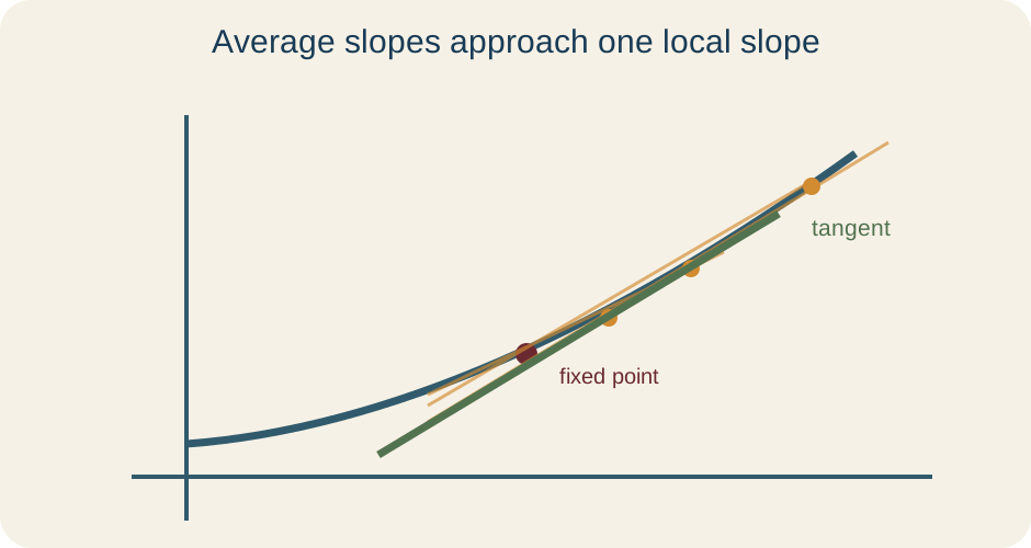
For a function $f$, the average rate of change from $x=a$ to $x=b$ is $\frac{f(b)-f(a)}{b-a}$. The numerator records output change. The denominator records input change. Their quotient measures output change per unit input change across the interval. Geometrically, it is the slope of the secant line through the two graph points.

Units carry the same interpretation. If $f(t)$ is position in meters and $t$ is time in seconds, the quotient uses meters per second. If cost is measured in dollars and production in items, the quotient uses dollars per item. A rate is not a bare number when its variables represent quantities. Units identify what is changing with respect to what.

Average change depends on both endpoints. A journey can have the same average velocity while containing very different motion histories. A nonlinear function can have different secant slopes on different intervals. To describe behavior at one input, the interval must shrink. Limits provide that passage from interval change to local change.

Build the instantaneous rate through a limit

Fix the first input at $x=a$ and write the second as $a+h$. The nonzero quantity $h$ is an input increment. The difference quotient is $\frac{f(a+h)-f(a)}{h}$. It measures average rate across the interval from $a$ to $a+h$. Letting $h$ approach zero asks whether these average rates settle on one value.

The derivative at $a$ is $f'(a)=\lim_{h\to0}\frac{f(a+h)-f(a)}{h}$ when the limit exists and is finite. The prime symbol marks a derivative. The limit does not substitute $h=0$ into the quotient because that would create division by zero. It examines nonzero increments that become arbitrarily small. The resulting value describes the function at the chosen input.

Both positive and negative increments matter at an interior point. Positive $h$ samples secants from the right, while negative $h$ samples from the left. Their limiting slopes must agree. If they approach different values, the function has no ordinary two-sided derivative there. One-sided derivatives may still describe the separate behaviors.

Derive a familiar power from first principles

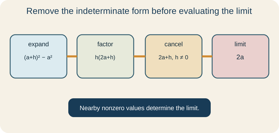
Let $f(x)=x^2$. The difference quotient at a general input $x$ is $\frac{(x+h)^2-x^2}{h}$. Expanding the square gives $\frac{x^2+2xh+h^2-x^2}{h}$. Combining opposite terms leaves $\frac{2xh+h^2}{h}$. Factoring and canceling the nonzero increment gives $2x+h$.

Now take the limit as $h$ approaches zero. The expression $2x+h$ approaches $2x$. Therefore the derivative function is $f'(x)=2x$. The cancellation occurred before the limit and only for nonzero $h$. This ordering resolves the apparent zero-over-zero form without dividing by zero.

The result has geometric meaning. At $x=3$, the parabola’s tangent slope is six. At negative three, the slope is negative six. At zero, the slope is zero and the graph has a horizontal tangent. One formula summarizes changing local behavior across the entire domain.

Unite tangent slope and instantaneous rate

On a graph of output versus input, the derivative is the tangent-line slope. A tangent line captures the graph’s first-order direction at one point. It is not defined merely as a line that touches once because some tangent lines cross their graphs. The limit of secant slopes supplies the robust definition. Geometry visualizes the same local ratio represented algebraically.

In a time model, that slope becomes an instantaneous rate. If $s(t)$ is position, then $s'(t)$ is velocity. The graph’s vertical units are meters and horizontal units are seconds, so tangent slope has meters-per-second units. The second derivative $s''(t)$ is acceleration with units meters per second squared. Graph and physical interpretations agree through units.

Other contexts use the same structure. A derivative of energy with respect to position has joules-per-meter units. A derivative of cost with respect to quantity has dollars-per-item units. A derivative of temperature with respect to distance has degrees-per-meter units. The variables change, but the local output-over-input interpretation remains fixed.

Interpret the derivative as sensitivity

Sensitivity asks how strongly an output responds to a small input change. A large derivative magnitude means a small input perturbation produces a relatively large first-order output change. A small magnitude means weaker local response. The sign indicates response direction. Positive derivatives associate increasing inputs with increasing outputs locally.

Sensitivity depends on units and scale. A derivative measured per meter will differ numerically from the same physical response measured per centimeter. Rescaling the input changes the numerical coefficient. Therefore derivative magnitude should never be interpreted without units. Comparisons require compatible variables and measurement scales.

Sensitivity can guide design and error analysis. If an instrument model is $y=f(x)$ and input uncertainty is approximately $\Delta x$, then output uncertainty is approximately $|f'(x)|\Delta x$. This is a local estimate rather than an exact identity. It becomes more reliable for smaller changes when the derivative varies smoothly. Curvature helps assess the neglected error.

See the derivative as local linearity

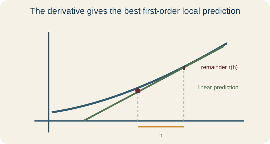
Differentiability means more than possessing a slope number. Near $x=a$, a differentiable function satisfies $f(a+h)=f(a)+f'(a)h+r(h)$, where the remainder $r(h)$ becomes negligible relative to $h$. Formally, $\frac{r(h)}{h}\to0$ as $h\to0$. The first two terms form the best local linear model. The remainder records nonlinear error.

Writing $x=a+h$ produces the familiar linearization $L(x)=f(a)+f'(a)(x-a)$. The value $f(a)$ anchors the line at the graph point. The derivative supplies its slope. The difference $x-a$ is the input displacement from the base point. The approximation is strongest near that base point.

For $f(x)=\sqrt{x}$ near $a=100$, the value is ten and the derivative is $\frac{1}{20}$. Thus $\sqrt{x}\approx10+\frac{1}{20}(x-100)$. At $x=101$, the estimate is $10.05$. Concavity shows that this tangent estimate is slightly high. The derivative has converted a nonlinear evaluation into a nearby linear calculation.

Distinguish derivative value from derivative function

The notation $f'(a)$ names one number: the derivative evaluated at the specific input $a$. The notation $f'(x)$ names a new function that assigns a derivative to each differentiable input. Deriving $f'(x)$ first allows later evaluation at many points. Computing directly at $a$ can be useful when only one local rate is needed. The two tasks should not be confused.

Leibniz notation provides another perspective. The symbol $\frac{dy}{dx}$ denotes the derivative of dependent quantity $y$ with respect to independent quantity $x$. The symbols suggest an output-change to input-change ratio. They are not generally ordinary fractions, although the notation supports chain-rule and unit reasoning. Context determines which variable is changing.

Operator notation $\frac{d}{dx}[f(x)]$ emphasizes the act of differentiation. It means apply the derivative operator with respect to $x$ to the enclosed expression. This notation is helpful when several variables appear. A derivative with respect to time treats other fixed parameters as constants. Naming the variable prevents ambiguous calculations.

Recognize when a derivative does not exist

A corner produces unequal finite one-sided slopes. The absolute-value function has left derivative negative one and right derivative positive one at zero. Because the values differ, no two-sided derivative exists there. The function remains continuous. Continuity alone is weaker than differentiability.

A cusp can produce unbounded slopes with opposite signs. A vertical tangent can produce unbounded slopes with a common geometric direction but no finite ordinary derivative. A discontinuity automatically prevents differentiability because differentiability implies continuity. Rapid oscillation can also keep secant slopes from settling. Each failure has distinct local evidence.

Domain endpoints may have one-sided derivatives. For a function defined only on $[a,\infty)$, a right derivative at $a$ can describe change from within the domain. Some courses reserve “differentiable at a point” for two-sided interior derivatives and name endpoint derivatives separately. State the convention being used. Domain-aware language avoids claiming nonexistent approaches.

Connect derivative sign to local behavior

A positive derivative indicates local increase, and a negative derivative indicates local decrease when interpreted across intervals with appropriate hypotheses. A zero derivative indicates a horizontal tangent candidate. It does not automatically prove a maximum or minimum. The function $f(x)=x^3$ has derivative zero at zero but continues increasing. Sign changes provide the classification.

Derivative magnitude measures steepness relative to the coordinate scales. A derivative near zero means the local graph is nearly horizontal. A large positive or negative value means a steep local line. Infinite-looking steepness does not represent a large finite derivative. A vertical tangent requires separate description.

The second derivative describes how the first derivative changes. Positive second derivative means slopes increase, giving concave-up behavior. Negative second derivative means slopes decrease, giving concave-down behavior. This adds information about how the local linear model evolves from point to point. Curvature also helps predict linearization error.

Use units to audit derivative calculations

Derivative units are output units divided by input units. If volume is measured in cubic meters and time in seconds, $\frac{dV}{dt}$ has units $\frac{\mathrm{m^3}}{\mathrm{s}}$. If pressure is measured in pascals and depth in meters, $\frac{dP}{dz}$ has units $\frac{\mathrm{Pa}}{\mathrm{m}}$. These fractional units communicate a rate. Omitting them removes part of the interpretation.

Suppose a spherical radius grows at $0.010\,\frac{\mathrm{m}}{\mathrm{s}}$ when $r=0.20\,\mathrm{m}$. With $V=\frac{4}{3}\pi r^3$, the chain rule gives $\frac{dV}{dt}=4\pi r^2\frac{dr}{dt}$. Substitution gives $4\pi(0.20\,\mathrm{m})^2(0.010\,\frac{\mathrm{m}}{\mathrm{s}})$. The result is $1.6\pi\times10^{-3}\,\frac{\mathrm{m^3}}{\mathrm{s}}$. The units confirm a volume rate.

Dimensional mismatch exposes missing factors. The quantity $4\pi r^2$ alone has square-meter units, so it cannot equal a volume-per-time rate. Multiplication by radial speed supplies the missing meters per second. This is exactly the chain rule’s sensitivity interpretation. Unit analysis acts as an independent structural check.

Separate symbolic, numerical, and graphical evidence

Symbolic differentiation produces an exact formula under stated assumptions. A numerical difference quotient estimates a derivative at a selected point. A graph visualizes tangent direction and rough magnitude. Each representation has different strengths. Agreement among them increases confidence.

To check $f'(a)$ numerically, compute $\frac{f(a+h)-f(a)}{h}$ for several positive and negative nonzero values of $h$. The estimates should approach a common value. Values of $h$ that are extremely small can suffer floating-point cancellation. A stable trend matters more than one apparently precise decimal. Numerical evidence supports but does not replace a proof.

Graphical scales can distort slope. Stretching the vertical axis makes a line look steeper without changing the underlying units-based derivative. A plotted cusp can appear smooth at low resolution. Use the graph to interpret and question the formula. Do not treat appearance alone as existence proof.

Diagnose common conceptual errors

One error substitutes $h=0$ before simplifying the difference quotient. The derivative limit uses nonzero increments approaching zero. Another error expands $f(x+h)$ incorrectly by replacing only one occurrence of $x$. Every occurrence must receive the grouped input $x+h$. Parentheses protect the substitution.

Another error treats the derivative as an average across a large interval. The derivative is a local limiting rate. An average rate may equal an instantaneous rate somewhere under the Mean Value Theorem, but the two are not generally identical at a chosen endpoint. State which interval or point each rate describes. Units alone cannot distinguish the scale.

A final error reports a slope without contextual meaning. A derivative answer should name the responding quantity, the changing input, the point of evaluation, the direction indicated by its sign, and the units. This sentence completes the mathematics. Interpretation is not optional decoration after calculation. It is the reason the calculation was performed.

Practice local-change reasoning

For $f(x)=x^2$, compute the average rate from two to $2+h$ and simplify before taking a limit. The quotient becomes $4+h$. Its limit is four, so the tangent slope at two is four. Check this value using the derivative function $f'(x)=2x$. Explain what positive slope means on the graph.

Next, let position be $s(t)=3t^2$ meters with time in seconds. Velocity is $s'(t)=6t$ meters per second. At $t=2.0$ seconds, velocity is $12\,\frac{\mathrm{m}}{\mathrm{s}}$. The positive sign indicates motion in the positive coordinate direction. Acceleration is $6\,\frac{\mathrm{m}}{\mathrm{s^2}}$.

For independent work, choose a nonlinear function and a safe base point. Estimate its derivative using difference quotients from both sides. Derive or obtain the symbolic derivative and compare. Construct the local linearization and test it at two nearby inputs. Describe how approximation error changes with distance from the base point.

Sources and further study

OpenStax Calculus, Volume 1 develops derivatives from tangent and rate problems. Its early differentiation chapters connect difference quotients with rules and applications. Re-derive one rule from the limit definition before using the shortcut. Track units in every contextual example. This practice keeps procedural fluency connected to meaning.

The AP Calculus AB course overview supplies curriculum alignment for derivative interpretations. It emphasizes graphical, numerical, analytical, and verbal representations. Translate one derivative value across all four. State assumptions and units in the verbal form. Representation changes reveal gaps that symbolic work can hide.

Further study should connect local linearity to multivariable derivatives and differential equations. In several variables, the derivative becomes a linear map rather than one slope. Differential equations prescribe local rates and ask which functions realize them. Numerical methods advance by repeated local approximations. The one-variable derivative is the foundation for all three developments.