Inverse Functions

An inverse function reverses a mapping by taking an output back to the input that produced it. Reversal is possible only when each relevant output identifies exactly one original input. That requirement links inverse functions to one-to-one behavior, domain restrictions, and composition. Graphically, inversion reflects ordered pairs across the line $y=x$. In applications, an inverse often converts a measurement back into the underlying quantity a model was designed to predict.

Begin with a reversible mapping

A function $f:A\to B$ assigns each input in set $A$ exactly one output in set $B$. The set $A$ is the domain. The set of outputs actually produced is the range. The codomain $B$ is the declared destination set and may be larger than the range. An inverse must know which outputs are intended as valid inputs for reversal.

Suppose $f$ sends $2$ to $7$. The inverse should send $7$ back to $2$. In ordered-pair notation, $(2,7)$ becomes $(7,2)$. Reversing every pair exchanges the roles of input and output. The reversed relation is a function only if no reversed input receives multiple outputs.

When $f$ is one-to-one from $A$ onto $B$, its inverse is written $f^{-1}:B\to A$. The superscript negative one labels inverse composition. It does not mean the reciprocal $1/f(x)$. Context and composition determine the notation’s meaning. This distinction must be explicit because exponent rules for numbers do not apply to function names in the same way.

Understand why one-to-one behavior matters

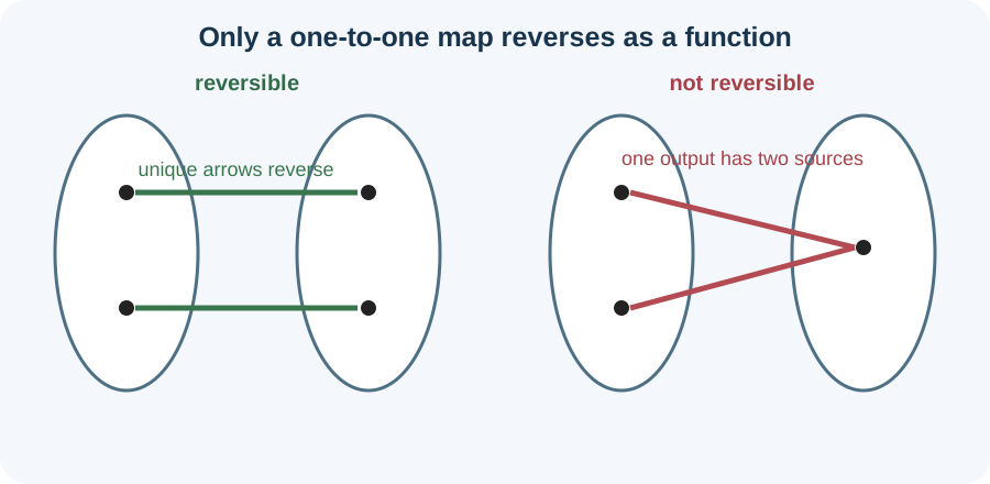
A function is one-to-one when different inputs always produce different outputs. Equivalently, $f(a)=f(b)$ implies $a=b$. This condition prevents an output from having two competing original inputs. Reversing the arrows then preserves the function rule. One-to-one behavior is also called injectivity.

The function $f(x)=x^2$ is not one-to-one on all real numbers. Both $2$ and $-2$ produce $4$. Reversal would ask the input $4$ to output both $2$ and $-2$. That reversed relation violates the rule that a function gives one output per input. The problem is not square-root notation; it is the original many-to-one mapping.

The function $g(x)=2x+3$ is one-to-one on the real numbers. If $2a+3=2b+3$, subtraction and division give $a=b$. Every output in its real range comes from exactly one input. Therefore reversing the map creates a valid function. Algebraic reasoning and mapping logic agree.

Apply the horizontal line test

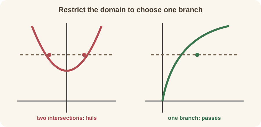
A graph represents a one-to-one function when every horizontal line intersects it at most once. A horizontal line represents one possible output value. Multiple intersections mean that output comes from multiple inputs. The test is therefore the graphical version of injectivity. It complements the vertical line test, which checks whether a relation is a function at all.

Any strictly increasing function is one-to-one on its interval. Any strictly decreasing function is also one-to-one. A function that turns around may still be one-to-one on selected pieces but not on the entire domain. Constant intervals immediately violate the condition. Graph shape provides a fast diagnostic before symbolic inversion.

The parabola $y=x^2$ fails because horizontal lines above zero meet it twice. Restricting the domain to $x\geq0$ leaves only the right branch. Each allowed horizontal line then meets the graph once. Restricting to $x\leq0$ would also work but would produce a different inverse branch. Domain choice is part of the inverse definition.

Restrict a domain deliberately

A domain restriction removes inputs so the remaining function becomes one-to-one. The restriction should be stated with the original formula. For $f(x)=x^2$ on $[0,\infty)$, the inverse is $f^{-1}(x)=\sqrt{x}$. For the same formula on $(-\infty,0]$, the inverse is $f^{-1}(x)=-\sqrt{x}$. The two branches reverse different original mappings.

A valid restriction should also fit the application. If $x$ represents a physical length, the nonnegative branch may already be natural. If $x$ represents a signed displacement known to be negative, the other branch may be appropriate. Algebra cannot choose the physical branch without context. A complete answer states both the restriction and its rationale.

Restricting a domain changes the function as a mapping even though its formula remains unchanged. The new range becomes the inverse’s domain. Values removed from the original range cannot be supplied to the inverse. Writing only an inverse formula without its domain loses essential information. Function identity includes rule, domain, and codomain or intended range.

Find an inverse algebraically

Begin by writing $y=f(x)$. Solve the equation for the original input $x$ in terms of output $y$. Then rename the new input variable as $x$ to use standard function notation. This procedure reverses roles rather than performing a magical symbol swap. The domain and range must be carried through the process.

Let $f(x)=\dfrac{3x-2}{5}$. Write $y=\dfrac{3x-2}{5}$. Multiplication gives $5y=3x-2$, so $x=\dfrac{5y+2}{3}$. Renaming the input yields $f^{-1}(x)=\dfrac{5x+2}{3}$. Both functions have real domain and real range.

The order of inverse operations becomes visible. The original function multiplies by three, subtracts two, and divides by five. Reversal multiplies by five, adds two, and divides by three. Inverse operations occur in reverse order. This operational view predicts the algebra and helps catch sign errors.

Verify both compositions and their domains

Inverse functions satisfy $f^{-1}(f(x))=x$ for every $x$ in the domain of $f$. They also satisfy $f(f^{-1}(y))=y$ for every $y$ in the domain of $f^{-1}$. The two equations describe opposite round trips. Each composition begins in one set and returns to that same set. Domain phrases are part of the identities.

For $f(x)=\dfrac{3x-2}{5}$, substitute into the inverse. The composition is $f^{-1}(f(x))=\dfrac{5((3x-2)/5)+2}{3}=x$. Reversing order gives $f(f^{-1}(x))=\dfrac{3((5x+2)/3)-2}{5}=x$. Both simplifications return the input. Agreement proves more than visual resemblance between formulas.

With restricted functions, a composition may simplify algebraically outside its valid domain but still lack meaning there. For $f(x)=x^2$ on $x\geq0$, $f^{-1}(f(x))=\sqrt{x^2}=|x|=x$ because $x$ is nonnegative. Without the restriction, $\sqrt{x^2}=|x|$ is not always $x$. Domain awareness explains the absolute value. A composition check should never silently expand the allowed inputs.

Exchange domain and range

The domain of $f^{-1}$ is the range of $f$. The range of $f^{-1}$ is the domain of $f$. This exchange follows because original outputs become inverse inputs. It also explains why inverse formulas may need restricted domains. The mapping sets reverse along with the ordered pairs.

For $f(x)=e^x$, the domain is all real numbers and the range is $(0,\infty)$. Its inverse is $\ln x$. Therefore logarithm has domain $(0,\infty)$ and real range. A logarithm of zero or a negative real number is outside this real inverse mapping. The restriction is structural rather than an arbitrary rule.

For $f(x)=\dfrac{1}{x-2}$, the domain excludes $2$, and the range excludes $0$. Solving $y=1/(x-2)$ gives $x=2+1/y$. Thus the inverse has domain excluding zero and range excluding two. The exclusions exchange exactly as predicted. Tracking them validates the inverse relationship.

Interpret inverse graphs as reflections

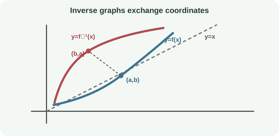
If $(a,b)$ lies on the graph of $f$, then $(b,a)$ lies on the graph of $f^{-1}$. Exchanging coordinates reflects points across line $y=x$. Points on the line remain fixed under this reflection. The original and inverse graphs therefore display symmetric shapes. Reflection provides a visual check, not a substitute for domain analysis.

The slopes also have a reciprocal relationship when derivatives exist and are nonzero. If the original graph has slope $m$ at $(a,b)$, the inverse has slope $1/m$ at $(b,a)$. Reflection exchanges horizontal and vertical changes. A horizontal tangent in the original may correspond to a vertical tangent in the inverse. This idea later becomes the inverse-function derivative formula.

Self-inverse functions have graphs symmetric with themselves across $y=x$. For example, $f(x)=1/x$ on nonzero real numbers is its own inverse. Composing it twice returns $x$. Not every symmetric-looking graph represents a function, so the vertical and horizontal line tests still apply. Mapping structure remains primary.

Distinguish an inverse from a reciprocal

The inverse function $f^{-1}(x)$ reverses input and output. The reciprocal $\dfrac{1}{f(x)}$ takes the original output and forms its multiplicative reciprocal. These are different operations. Their domains and graphs generally differ. Similar notation should not be allowed to merge their meanings.

For $f(x)=2x$, the inverse is $f^{-1}(x)=x/2$. The reciprocal is $1/(2x)$. Composing the inverse with $f$ returns $x$. Multiplying the reciprocal by $f(x)$ returns one wherever defined. These distinct identities reveal which operation is present.

The notation $\sin^{-1}x$ can be especially ambiguous. In most precalculus contexts it means $\arcsin x$, the inverse sine function. The reciprocal of sine is $\csc x$, not arcsine. Clear writing favors $\arcsin$ when confusion is possible. Readers should infer meaning from function composition and domain, not exponent appearance alone.

Reverse units and calibration models

An applied function often converts one kind of quantity into another. Suppose $F(C)=\dfrac95C+32$ converts degrees Celsius to degrees Fahrenheit. Its input unit is degrees Celsius, and its output unit is degrees Fahrenheit. The inverse must accept Fahrenheit values and return Celsius values. Solving gives $C(F)=\dfrac59(F-32)$.

The coefficient $9/5$ is a ratio of temperature-scale increments, not a unit-free permission to mix scales carelessly. The offset $32$ has Fahrenheit-scale meaning. The inverse subtracts the offset before rescaling. For $F=68.0\,^{\circ}\mathrm F$, the result is $C=\dfrac59(68.0-32.0)=20.0\,^{\circ}\mathrm C$. Units accompany the input, intermediate difference, and output interpretation.

A calibration function may map concentration to instrument signal. Its inverse maps measured signal back to estimated concentration. If the calibration is not one-to-one over the working range, a measured signal does not identify one concentration. Restricting the operating range or adding another measurement may restore identifiability. Inverse-function conditions therefore have practical experimental consequences.

Understand exponential and logarithmic inversion

For base $b>0$ with $b\neq1$, exponential function $f(x)=b^x$ is one-to-one. Its range is positive real numbers. The inverse is logarithm base $b$, written $f^{-1}(x)=\log_bx$. The identity $\log_b(b^x)=x$ holds for every real $x$. The identity $b^{\log_bx}=x$ holds for positive $x$.

The logarithm answers an exponent question. The equation $b^y=x$ is equivalent to $y=\log_bx$. This equivalence is the inverse relationship in symbolic form. It explains logarithm rules as translations of exponent rules. Domain restrictions follow because positive-base exponentials never output zero or negative values.

For $e^{kt}=A$ with positive $A$, applying natural logarithm gives $kt=\ln A$. Then $t=\dfrac{\ln A}{k}$ when $k\neq0$. The logarithm reverses the exponential after its argument is isolated. A common error is taking logarithms of only one term in a sum. Inversion applies to the complete exponential output, not selectively to pieces.

Define inverse trigonometric branches

Periodic trigonometric functions are not one-to-one on all real numbers. Sine repeats every $2\pi$ radians. Cosine and tangent also repeat. To create inverse functions, standard domains are restricted to intervals covering one suitable branch. The selected inverse returns a principal angle.

Sine is restricted to $[-\dfrac{\pi}{2},\dfrac{\pi}{2}]$ for $\arcsin$. Its inverse domain is $[-1,1]$, the range of sine. The output range of arcsine is the selected angle interval. Thus $\arcsin(1/2)=\pi/6$, even though infinitely many angles have sine one-half. The inverse returns one principal value rather than all solutions to a trigonometric equation.

Cosine is conventionally restricted to $[0,\pi]$ for $\arccos$. Tangent is restricted to $(-\pi/2,\pi/2)$ for $\arctan$. These choices make each function one-to-one while preserving a useful continuous branch. Different branches could be selected, but conventions support consistent communication. Solving a trigonometric equation still requires finding all angles demanded by the problem, not only the principal inverse value.

Solve equations using inverse functions

If $f$ is one-to-one and $f(x)=c$, applying $f^{-1}$ to both sides gives $x=f^{-1}(c)$. This operation is valid when $c$ lies in the range of $f$. The inverse undoes the entire function. It does not distribute across sums or products unless a separate algebraic rule justifies doing so. Isolate the function output before inversion.

For $3e^{2x}-4=8$, first add four and divide by three to obtain $e^{2x}=4$. Apply natural logarithm to get $2x=\ln4$. Then $x=\dfrac{\ln4}{2}=\ln2$. Substitution into the original equation verifies the result. Every step preserves equivalence because the isolated exponential is positive.

For a square restricted to nonnegative inputs, solving $x^2=9$ through its inverse gives $x=3$. Without that domain restriction, the equation has both $x=3$ and $x=-3$. Inverse-function solving inherits the mapping’s domain. Apparent loss of a root often reflects an unstated branch choice. Listing the original domain makes the selected answer logically transparent.

Diagnose common inverse errors

One error is writing $f^{-1}=1/f$. Another is swapping $x$ and $y$ but failing to solve for the new output. A third is ignoring one-to-one behavior. A fourth is omitting domain and range. Each error confuses symbolic manipulation with reversal of a mapping.

Composition is the strongest algebraic check. Compute both orders when domains are not obvious. Graph reflection provides a geometric check. Domain-range exchange provides a set-based check. Agreement among all three exposes a valid inverse more convincingly than pattern recognition.

Calculator inverse keys can hide principal-value restrictions. An arcsine result is one selected angle. A numerical inverse of a calibration curve may depend on a chosen interval. Software may also report complex values outside a real domain. State the intended number system and branch before interpreting output.

Practice and connect forward

Find the inverse of $f(x)=4x+7$. Solve $y=4x+7$ for $x$ to obtain $x=(y-7)/4$. Therefore $f^{-1}(x)=\dfrac{x-7}{4}$. Verify both compositions. State that both domain and range are all real numbers.

Restrict $g(x)=(x-2)^2$ so its inverse is $g^{-1}(x)=2+\sqrt{x}$. The chosen original domain is $x\geq2$. Its range is $x\geq0$, which becomes the inverse domain. Reflect representative points across $y=x$. Explain why the negative square-root branch corresponds to a different original restriction.

Inverse ideas continue into calculus. Differentiating $f(f^{-1}(x))=x$ produces the derivative rule for inverse functions. Logarithmic differentiation relies on exponential-logarithmic inversion. Inverse trigonometric derivatives inherit their branch domains. A clear mapping foundation keeps those later formulas connected to meaning.