Polynomial and Rational Behavior

Polynomial and rational graphs contain more structure than a table of sampled points reveals. A leading term predicts distant behavior, factors reveal zeros and excluded inputs, and multiplicity predicts whether signs change. Rational functions add holes and asymptotes that must be distinguished through cancellation and limits. Sign charts connect the algebraic factors to graph regions. This lesson develops a systematic graph analysis that can later be made precise with calculus.

Read a polynomial from its algebraic forms

A polynomial has form $P(x)=a_nx^n+a_{n-1}x^{n-1}+\cdots+a_1x+a_0$, where $a_n\neq0$. The nonnegative integer $n$ is the degree. The coefficient $a_n$ is the leading coefficient. Expanded form makes degree and leading term visible. Factored form makes zeros and multiplicities visible.

No single algebraic form is best for every question. The polynomial $x^3-3x^2-4x+12$ reveals its leading term in expanded form. Factoring by grouping gives $(x-3)(x-2)(x+2)$, which reveals three zeros. Both expressions define the same function. Moving between forms exposes different graph features without changing the mapping.

The constant term $a_0=P(0)$ gives the vertical-axis intercept. A factor $x-r$ gives horizontal-axis intercept $r$. Degree places an upper bound on the number of real zeros and turning points. It does not guarantee that every possible zero or turn occurs. Structural predictions should be treated as constraints rather than a complete graph by themselves.

Predict polynomial end behavior

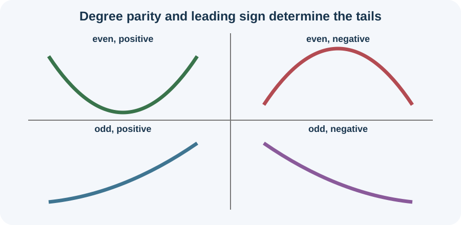
For large $|x|$, the leading term $a_nx^n$ dominates lower powers. The notation $|x|$ means distance from zero, so large absolute value includes both far-left and far-right inputs. Lower-degree terms become small relative to $x^n$. End behavior therefore follows the leading coefficient and degree parity. This is an asymptotic statement rather than an equality at finite inputs.

When $n$ is even, $x^n$ is positive on both ends. A positive leading coefficient makes both ends rise, while a negative coefficient makes both fall. When $n$ is odd, $x^n$ changes sign from left to right. A positive leading coefficient produces left down and right up. A negative leading coefficient reverses those directions.

For $P(x)=-3x^5+2x$, the leading term is $-3x^5$. As $x\to\infty$, the polynomial tends to $-\infty$. As $x\to-\infty$, it tends to $\infty$. The arrow notation means that inputs move without bound in the stated direction. It describes graph tails and does not claim an infinite value is ever reached.

Interpret zeros through factorization

A zero $r$ satisfies $P(r)=0$. By the factor theorem, this occurs exactly when $x-r$ is a factor. On the graph, a real zero is an $x$-intercept. Factoring transforms an equation-solving question into visible product structure. Substitution verifies every proposed root.

Suppose $P(x)=2(x+1)(x-3)^2$. Its zeros are $x=-1$ and $x=3$. The leading coefficient is two, not one, because the highest-degree product is $2x^3$. The degree is three because factor exponents add. The vertical intercept is $P(0)=2(1)(9)=18$.

A polynomial of degree $n$ has exactly $n$ complex zeros counted with multiplicity, according to the fundamental theorem of algebra. Some may be nonreal and therefore do not appear as horizontal-axis crossings. Real-coefficient polynomials have nonreal roots in conjugate pairs. Graph analysis focuses on real zeros while algebra retains the broader count. This distinction explains why an even-degree polynomial can have no real intercepts.

Use multiplicity to predict local crossing behavior

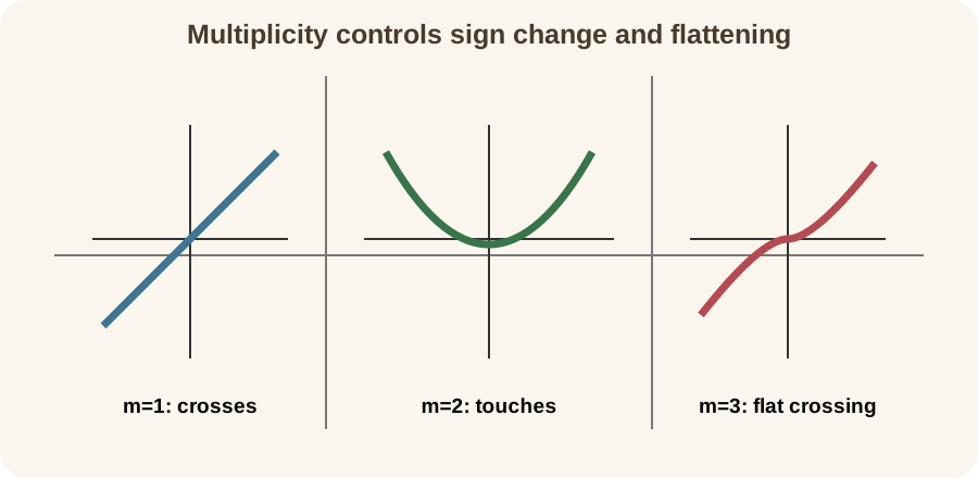
If $P(x)=a(x-r)^mQ(x)$ with $Q(r)\neq0$, then zero $r$ has multiplicity $m$. The exponent counts repeated copies of factor $x-r$. Odd multiplicity makes the factor change sign across $r$. Even multiplicity preserves its sign. The complete polynomial may include other factors, but their signs remain locally fixed near $r$.

An odd-multiplicity zero generally crosses the horizontal axis. An even-multiplicity zero touches the axis and turns back. Greater multiplicity also produces more local flattening. A simple zero with $m=1$ usually crosses sharply. A triple zero crosses with a flattened shape.

For $P(x)=2(x+1)(x-3)^2$, the zero $-1$ has odd multiplicity one and the graph crosses there. The zero $3$ has even multiplicity two and the graph touches without changing sign. Since total degree is three and leading coefficient positive, the left tail falls and right tail rises. These features provide a skeleton before any additional points are plotted. Evaluating the vertical intercept adds one reliable anchor to that skeleton.

Build a polynomial sign chart

A sign chart divides the real line at each real zero. Inside any interval containing no zeros, a continuous polynomial cannot change sign. Choose one test point per interval and determine the product sign. At odd-multiplicity zeros, the sign changes. At even-multiplicity zeros, it stays the same.

For $P(x)=2(x+1)(x-3)^2$, critical values are $-1$ and $3$. The squared factor is nonnegative and positive away from three. Therefore the sign is controlled by $x+1$ except at the zeros. The polynomial is negative for $x<-1$ and positive for $x>-1$ except that it equals zero at three. This result matches the multiplicity prediction.

Sign charts are more reliable than plotting many random points. They identify where the graph lies above or below the axis. Combined with intercepts and end behavior, they constrain the overall shape. They do not locate exact turning points. Calculus later uses derivatives for that finer information.

Define rational functions and their domains

A rational function has form $R(x)=\dfrac{P(x)}{Q(x)}$, where $P$ and $Q$ are polynomials and $Q$ is not the zero polynomial. Its domain excludes every real input satisfying $Q(x)=0$. The horizontal fraction bar means the entire polynomial $P(x)$ is divided by the entire polynomial $Q(x)$. Parentheses should preserve that grouping when formulas are entered into software. Domain exclusions exist before any cancellation.

For $R(x)=\dfrac{x^2-9}{(x-3)(x-1)}$, denominator zeros are three and one. Both values are excluded from the original domain. Factoring the numerator gives $(x-3)(x+3)$. The factor $x-3$ can cancel algebraically for allowed inputs. Cancellation does not restore the excluded point $x=3$.

The simplified expression is $(x+3)/(x-1)$ with condition $x\neq3$. It agrees with the original at every shared domain input. At $x=3$, the simplified rule would output three, but the original function remains undefined. This missing point creates a hole. Writing the restriction beside the simplified formula preserves the original mapping.

Distinguish holes from vertical asymptotes

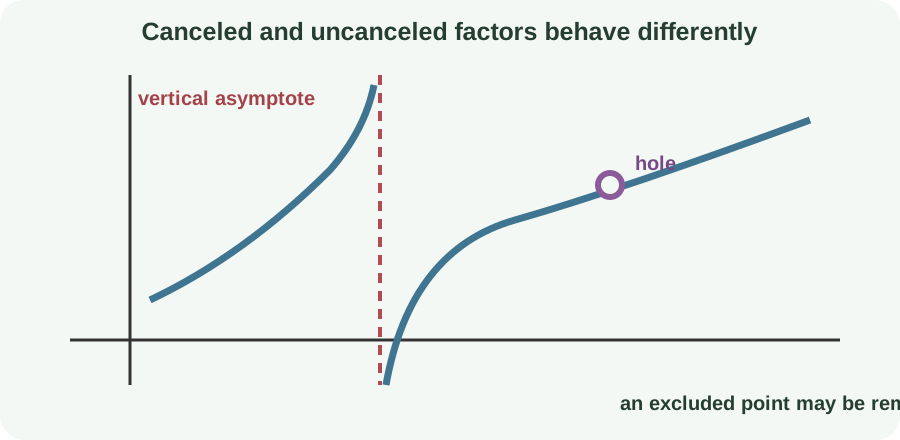
A canceled denominator factor creates a removable discontinuity when the remaining expression has a finite value at that input. The graph has a hole at the corresponding point. The hole’s vertical coordinate is found by evaluating the reduced expression. The term removable means a new definition at that single point could make the function continuous. It does not mean ordinary cancellation already filled the point.

An uncanceled denominator zero is a candidate for a vertical asymptote. Near such an input, the function magnitude often grows without bound. One-sided signs can differ. A vertical asymptote has equation $x=a$, where $a$ is an input value. Substitution alone gives division by zero but does not fully describe nearby behavior.

For $R(x)=\dfrac{x^2-9}{(x-3)(x-1)}$, there is a hole at $x=3$. The reduced value there would be $(3+3)/(3-1)=3$, so the hole is $(3,3)$. The uncanceled denominator factor $x-1$ produces a vertical asymptote at $x=1$. Keeping the two excluded values separate prevents the mistake of calling every denominator zero an asymptote. A domain table should record both exclusions even though their graph behaviors differ.

Analyze one-sided behavior near vertical asymptotes

Factored form reveals signs near an uncanceled denominator zero. Write every factor and determine which change sign across the critical input. A factor with odd multiplicity changes sign. A factor with even multiplicity does not. The numerator’s local sign also affects whether branches approach positive or negative infinity.

Consider $R(x)=\dfrac{1}{x-2}$. Just left of two, the denominator is a small negative number, so the quotient is a large negative number. Just right of two, it is a small positive number, so the quotient is large and positive. Symbolically, $R(x)\to-\infty$ as $x\to2^-$ and $R(x)\to\infty$ as $x\to2^+$. Superscripts minus and plus indicate approach from the left and right.

For $R(x)=1/(x-2)^2$, both sides produce a small positive denominator. Both branches therefore approach positive infinity. Even denominator multiplicity preserves sign across the asymptote. This mirrors even-multiplicity behavior at polynomial zeros, but the magnitude now diverges because the factor is downstairs. Factor location changes zero behavior into reciprocal blow-up behavior.

Determine horizontal end behavior by degree

For $R(x)=P(x)/Q(x)$, compare numerator degree $n$ with denominator degree $m$. If $n<m$, then $R(x)\to0$ as $x\to\pm\infty$, so $y=0$ is a horizontal asymptote. The denominator grows faster in magnitude. Lower-degree terms do not change this limiting ratio. The graph may still cross the asymptote at finite inputs.

If $n=m$, the horizontal asymptote is the ratio of leading coefficients. Divide numerator and denominator by $x^n$ to see why. Lower-power ratios approach zero as $|x|$ grows. For $R(x)=\dfrac{4x^2+1}{2x^2-5x}$, the asymptote is $y=4/2=2$. This is a limiting value rather than a forbidden output.

If $n>m$, there is no horizontal asymptote from a finite constant ratio. Polynomial division reveals a polynomial asymptote instead. When degree difference is one, that asymptote is a line called a slant or oblique asymptote. Larger degree differences produce higher-degree polynomial asymptotes. The remainder divided by $Q(x)$ approaches zero when its degree is smaller than the denominator degree.

Find a slant asymptote by division

Suppose $R(x)=\dfrac{x^2+1}{x-1}$. Polynomial division gives $R(x)=x+1+\dfrac{2}{x-1}$. The quotient $x+1$ is the candidate slant asymptote. The remainder term approaches zero as $|x|$ increases. Therefore the graph approaches line $y=x+1$.

The graph can cross a slant asymptote when the remainder term equals zero. In this example, the numerator of the remainder is constant two, so it never crosses the line at a finite domain input. Other rational functions can cross their polynomial asymptotes. The word asymptote describes limiting separation. It does not impose an uncrossable wall.

Division also clarifies graph deviations. The sign of remainder term tells whether the rational graph lies above or below the asymptote. Near a vertical asymptote, the remainder term may dominate. Far away, it becomes small. One decomposition therefore explains both local and distant behavior.

Build a rational sign chart

Factor numerator and denominator completely over the real numbers when possible. Mark numerator zeros, denominator zeros, and canceled exclusions on one number line. These critical values divide the domain into intervals. Test one point in each interval. Multiplicity predicts which signs change when a boundary is crossed.

For $R(x)=\dfrac{(x-1)^2}{(x+2)(x-4)}$, critical values are $-2$, $1$, and $4$. The numerator is nonnegative and vanishes with even multiplicity at one. Each denominator factor has odd multiplicity and changes sign at its zero. The function is positive on $(-\infty,-2)$, negative on $(-2,1)$ and $(1,4)$, and positive on $(4,\infty)$. There is no sign change at the even numerator zero.

The sign chart predicts graph location relative to the axis. The function touches the axis at $x=1$. It diverges near $x=-2$ and $x=4$. Horizontal end behavior approaches the ratio of leading coefficients, which is one. Combining these facts yields a coherent graph skeleton.

Construct a graph in a reliable order

Begin by state the domain and factor the expression. Mark holes, intercepts, and vertical asymptotes. Determine end behavior or polynomial asymptotes. Build a sign chart. Only then add a few strategically chosen points.

Near each vertical asymptote, use one-sided signs to orient branches. At each zero, use multiplicity to decide crossing or touching. At a hole, draw an open point at the reduced-function value. At the tails, approach the appropriate asymptote. These local rules must agree on every interval.

A graphing utility can verify the sketch but should not replace analysis. Its viewing window may hide holes or make distant behavior appear flat. Pixel sampling can connect across an asymptote incorrectly. Plot excluded points and asymptotes explicitly when possible. Structural knowledge tells the user when software output is misleading.

Interpret polynomial and rational models

Polynomial models are smooth for every real input. They can approximate behavior well on a finite interval but may grow unrealistically outside it. Leading terms dominate extrapolation. A high-degree fit can oscillate between data points. Model interpretation should remain tied to the range of evidence.

Rational models can represent saturation, resonance-like response, rates, and competing growth scales. Denominator zeros may indicate real singular behavior or simply a model boundary where assumptions fail. Horizontal asymptotes can represent limiting response. Holes may arise from algebraic construction rather than physical impossibility. Context determines whether a mathematical feature is meaningful.

Units constrain rational formulas. Terms added within a polynomial must have compatible units after coefficients are included. A ratio’s output units come from numerator units divided by denominator units. An asymptote inherits output units. Dimensional analysis can expose an apparently valid formula that cannot represent the claimed quantity.

Diagnose common mistakes

One mistake is treating every denominator zero as a vertical asymptote. Factor and cancel while preserving exclusions. Another is assuming a graph cannot cross a horizontal asymptote. Asymptotes describe limits, not barriers. A third is predicting all graph details from the leading term.

Multiplicity is also frequently ignored. Without it, a sketch may cross where it should touch. A sign chart should include repeated factors rather than only distinct critical numbers. Hole coordinates should come from the reduced expression. Substituting into the original undefined formula cannot produce them.

Fraction notation must preserve grouping. Write $\dfrac{P(x)}{Q(x)}$ with a horizontal bar in mathematical expressions. When entering plain text into software, use parentheses around both polynomials. An omitted parenthesis changes the function. Good notation prevents a formatting choice from becoming an algebra error.

Practice a complete structural analysis

Analyze $P(x)=-3x^5+2x$. Factor it as $x(2-3x^4)$ to find real zeros. Determine multiplicities and construct a sign chart. Use the negative odd leading term for end behavior. Then compare a hand sketch with a plotting tool.

Analyze $R(x)=\dfrac{x^2-9}{(x-3)(x-1)}$. State original domain exclusions before cancellation. Identify the hole and vertical asymptote. Find the horizontal asymptote from equal leading degrees. Use signs to orient branches on each interval.

Finally analyze $S(x)=\dfrac{x^2+1}{x-1}$. Perform polynomial division and state the slant asymptote. Determine the vertical asymptote and one-sided behavior. Find the vertical intercept and note that there are no real numerator zeros. Assemble these facts into a labeled graph without relying on random point tables.

Connect forward to limits and derivatives

Precalculus structure predicts what calculus later states precisely. End behavior becomes a limit as $x$ approaches positive or negative infinity. Vertical asymptotes become infinite one-sided limits. Holes become removable discontinuities with finite limits. Asymptotic language gains formal definitions.

Derivatives locate intervals of increase, decrease, concavity, and exact turning points. Polynomial degree bounds possible derivative zeros. Rational derivatives combine numerator and denominator structure through the quotient rule. The sign-chart habit carries directly into derivative analysis. Algebra remains part of calculus rather than being replaced by it.

You are ready to continue when you can move between expanded and factored forms, interpret multiplicity, and construct sign charts. You should distinguish holes from vertical asymptotes and limiting behavior from prohibited crossings. You should use polynomial division and degree comparison to find end behavior. These skills create a defensible graph before technology or calculus refines it. Limits and derivatives can then formalize predictions already grounded in structure.