Transformations of Functions

A function accepts an input and produces an output. A graph records all ordered pairs that make this relationship true. A transformation changes what input the function receives, what happens to its output, or both. Those two locations in an expression create different geometric effects. Understanding the input–output chain makes the rules predictable.

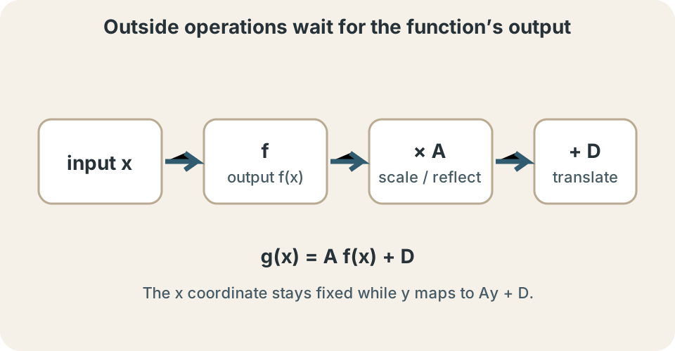
Expressions outside the function act on outputs after evaluation. Expressions inside the function alter which original input is sampled. This timing explains why vertical changes often look direct while horizontal changes appear reversed or reciprocal. The apparent reversal is not a trick. It follows from solving for the new input location.

This lesson derives translations, reflections, stretches, compressions, and combined mappings. It also tracks key points, domains, ranges, intercepts, asymptotes, and periodic features. Diagrams connect algebraic location with geometric motion. Worked examples retain exact horizontal fractions. The goal is to reason from function meaning rather than memorize a chart.

Learning goals and an opening comparison

You should distinguish an inside change from an outside change. You should predict graph movement from equations and derive horizontal effects. You should map key points through combined transformations. You should update domain, range, intercept, and asymptote information. You should also identify when transformation order changes the final function.

Compare $g(x)=f(x)+3$ with $h(x)=f(x+3)$. The first adds three after $f$ produces an output. Every output therefore rises by three. The second asks $f$ to evaluate an input three greater than the displayed $x$. Existing features appear three units earlier, so the graph shifts left.

This contrast is the central puzzle. The same visible $+3$ produces different effects because it occupies a different place in the input–output process. Predict the changed coordinate before using a rule. Then verify with one known point. A test point often exposes a reversed horizontal interpretation.

A graph is a set of input–output pairs

If $(u,v)$ lies on the graph of $f$, then $v=f(u)$. The symbol $u$ represents an original input. The symbol $v$ represents its original output. Transformations can map this pair to a new pair. Point mapping provides a general derivation method.

Suppose $f(2)=5$. Then $(2,5)$ belongs to the graph. For $g(x)=f(x)+4$, substituting $x=2$ gives $g(2)=9$. The input stays two while the output changes to nine. The point maps from $(2,5)$ to $(2,9)$.

For $h(x)=f(x-3)$, find the new input that feeds the old value $2$ into $f$. Solve $x-3=2$, giving $x=5$. Therefore $h(5)=f(2)=5$. The old point $(2,5)$ maps to $(5,5)$. Its output remains unchanged during this horizontal translation.

Outside addition translates outputs vertically

For $g(x)=f(x)+D$, constant $D$ is added to every output. The input is unchanged. If $(u,v)$ lies on $f$, then $(u,v+D)$ lies on $g$. Positive $D$ shifts upward. Negative $D$ shifts downward.

The letter $D$ can represent any real constant. In $g(x)=f(x)-6$, write $D=-6$. Every $y$ coordinate decreases by six. Vertical distances between graph points remain unchanged. The graph’s shape and orientation are preserved.

Vertical translation changes range values by $D$. It usually changes a horizontal asymptote $y=L$ into $y=L+D$. Domain stays unchanged because the function receives the same inputs. Vertical intercepts may change. Horizontal intercepts usually require solving a new equation.

Outside multiplication scales and reflects outputs

For $g(x)=Af(x)$, every output is multiplied by $A$. A point $(u,v)$ maps to $(u,Av)$. If $|A|>1$, vertical distances from the $x$ axis grow. If $0<|A|<1$, those distances shrink. Absolute value $|A|$ gives the vertical scale factor.

If $A<0$, output signs reverse. The graph reflects across the $x$ axis in addition to scaling by $|A|$. A point above the axis moves below it. Points on the $x$ axis remain fixed because zero multiplied by $A$ is zero. The order “scale then reflect” or “reflect then scale” gives the same result for this origin-centered output operation.

For $g(x)=-2f(x)$, point $(3,-4)$ maps to $(3,8)$. Multiplication gives $(-2)(-4)=8$. Its distance from the $x$ axis doubles. Its side of the axis reverses. This one point confirms both effects.

Inside translation changes sampled inputs

Consider $h(x)=f(x-C)$. To reproduce the old output $f(u)$, require $x-C=u$. Solving gives $x=u+C$. Therefore old point $(u,v)$ maps to $(u+C,v)$. Positive $C$ shifts the graph right.

Expression $f(x+4)$ can be written $f[x-(-4)]$. Here $C=-4$, so the graph shifts left four. The visible sign appears opposite the geometric direction because the equation is solved for the new coordinate. Calling this a “backward rule” hides the reason. Input matching explains it.

Check with the parent point $f(0)=0$ for $f(x)=x^2$. In $h(x)=(x-3)^2$, the zero output occurs when $x-3=0$, so $x=3$. The vertex moves from $(0,0)$ to $(3,0)$. Direct substitution verifies the rightward shift. The test point makes the direction unambiguous.

Inside multiplication uses a reciprocal scale

For $h(x)=f(Bx)$, reproduce old input $u$ by solving $Bx=u$. The new coordinate is $x=\frac{u}{B}$. Thus $(u,v)$ maps to $\left(\frac{u}{B},v\right)$. Horizontal coordinates are divided by $B$. The scale magnitude is $\frac{1}{|B|}$.

If $|B|>1$, coordinates move closer to the $y$ axis, creating horizontal compression. If $0<|B|<1$, coordinates move farther away, creating horizontal stretch. This reciprocal behavior comes from input matching. The graph changes which displayed input reaches each old function value. It is not the same as multiplying output.

For $h(x)=f(2x)$, an old point at input $6$ appears at new input $\frac{6}{2}=3$. The graph is horizontally compressed by $\frac{1}{2}$. For $h(x)=f\left(\frac{x}{3}\right)$, solve $\frac{x}{3}=u$ to get $x=3u$. That graph stretches horizontally by three. Both outcomes follow from matching the parent input.

Negative inside factors reflect across the y-axis

For $h(x)=f(-x)$, old input $u$ occurs when $-x=u$. Therefore $x=-u$. Point $(u,v)$ maps to $(-u,v)$. Horizontal signs reverse while outputs stay the same. This is reflection across the $y$ axis.

For general $f(Bx)$ with $B<0$, two effects occur. Division by $|B|$ gives horizontal scaling. The negative sign reverses horizontal direction. A point on the $y$ axis remains fixed. The combined map is still $x=\frac{u}{B}$.

Even functions satisfy $f(-x)=f(x)$, so a $y$-axis reflection leaves their graph unchanged. Odd functions satisfy $f(-x)=-f(x)$, linking horizontal and vertical reflection. Symmetry can hide a transformation visually. Algebraic comparison confirms whether two formulas are equivalent. An unchanged picture does not mean no transformation was applied.

Combined transformation form

A useful general form is $g(x)=Af[B(x-C)]+D$. Inside constants $B$ and $C$ alter inputs. Outside constants $A$ and $D$ alter outputs. The parent function $f$ supplies the original graph. Brackets show the full input expression.

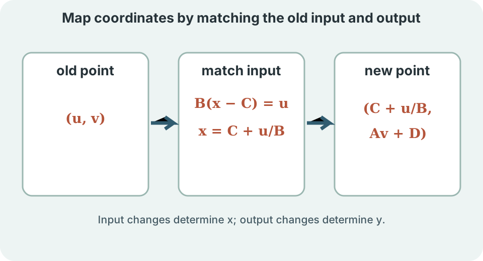
To map old point $(u,v)$, solve $B(x-C)=u$. Dividing by $B$ gives $x-C=\frac{u}{B}$. Adding $C$ gives $x=C+\frac{u}{B}$. The new output is $y=Av+D$. This derivation assumes $B\ne0$.

Therefore the point map is $\left(u,v\right)\mapsto\left(C+\frac{u}{B},Av+D\right)$. This single relationship handles translations, reflections, and scaling. It also preserves the difference between input and output changes. Substitution back into $g$ verifies the map. Every parent point is processed by the same coordinate rule.

Worked example with a parabola

Start with parent $f(x)=x^2$ and consider $g(x)=-2(x-3)^2+5$. Match it to $Af[B(x-C)]+D$. Here $A=-2$, $B=1$, $C=3$, and $D=5$. The vertex parent point is $(0,0)$. Mapping gives $(3,5)$.

The positive $C=3$ shifts right three. Magnitude $|A|=2$ stretches vertically by two. Negative $A$ reflects across the $x$ axis. Constant $D=5$ shifts up five. No horizontal scale or reflection occurs because $B=1$.

The parent range is $[0,\infty)$. Multiplication by $-2$ reverses it to $(-\infty,0]$. Addition of five produces $(-\infty,5]$. Domain remains all real numbers. The mapped vertex and range agree with a downward-opening parabola.

Mapping several key points

One point establishes a feature but not an entire curve. Choose a small parent table with distinctive inputs. For $f(x)=x^2$, useful points include $(-2,4)$, $(-1,1)$, $(0,0)$, $(1,1)$, and $(2,4)$. Transform each using the same map. Plot the mapped points before sketching.

For $g(x)=-2(x-3)^2+5$, map $(1,1)$ to $(4,3)$. Map $(-1,1)$ to $(2,3)$. These symmetric points confirm the axis $x=3$. Map $(2,4)$ to $(5,-3)$. Map $(-2,4)$ to $(1,-3)$.

The mapped table preserves connections among points. It also reveals vertical scale and reflection numerically. Avoid applying a different verbal sequence to each point. One algebraic map controls them all. A smooth curve should pass through the transformed points while retaining the parent’s qualitative structure.

Domain transforms through the input condition

If parent $f$ has domain set $S$, then $f[B(x-C)]$ is defined when $B(x-C)\in S$. This membership statement means the transformed input must be an allowed parent input. Outside multiplication and addition do not usually change domain. Inside changes can translate, scale, or reflect it. Solve the condition algebraically.

For $g(x)=\sqrt{2(x-4)}$, the square-root input must satisfy $2(x-4)\geq0$. Division by positive two gives $x-4\geq0$. Therefore $x\geq4$. The domain is $[4,\infty)$. Bracket notation includes the endpoint because zero has a defined square root.

For $h(x)=\frac{1}{3-x}$, the denominator cannot equal zero. Solve $3-x\ne0$, giving $x\ne3$. The negative inside coefficient reflects and shifts the parent reciprocal graph. Algebraic restriction identifies the excluded input exactly. A sketch should confirm rather than replace the condition.

Range transforms through outputs

If parent range is set $R$, then transformed outputs have form $Ay+D$ for $y\in R$. A positive $A$ preserves range order. A negative $A$ reverses inequalities. Constant $D$ shifts all range values. The input transformation does not change which parent output values occur when its input map covers the parent domain.

Suppose $f$ has range $[2,\infty)$ and $g(x)=-3f(x)+1$. Multiplying by $-3$ turns values into $(-\infty,-6]$. Adding one gives $(-\infty,-5]$. The endpoint $2$ maps to $-3(2)+1=-5$. The inequality direction changes because the scale factor is negative.

For restricted domains, an inside transformation can indirectly affect realized outputs if not every parent input remains available. The general set condition should then be used carefully. Do not update range by a slogan alone. Identify what outputs actually occur. Mapping critical points helps.

Intercepts require separate checks

The $y$ intercept occurs at displayed input $x=0$. For $g(x)=Af[B(x-C)]+D$, compute $g(0)=Af(-BC)+D$. It is not generally obtained by shifting the old $y$ intercept alone because inside transformations move which parent input lies on the $y$ axis. Direct substitution is reliable. The resulting point has coordinate form $(0,g(0))$.

An $x$ intercept satisfies $g(x)=0$. Solve $Af[B(x-C)]+D=0$. If $A\ne0$, this requires $f[B(x-C)]=-\frac{D}{A}$. The transformed zeros may therefore come from parent points whose output is not zero. Vertical translation changes zero locations.

In contrast, if $D=0$ and $A\ne0$, outside scaling alone preserves the parent zeros. Inside changes relocate them through the input map. Distinguish a zero from a $y$ intercept. Both are intercepts, but they solve different conditions. Label axes and equations.

Asymptotes and discontinuities transform too

A vertical asymptote at parent input $u=a$ maps through $B(x-C)=a$. Its new location is $x=C+\frac{a}{B}$. Vertical scaling and translation do not change that input location. The graph’s behavior on each side may reflect. Domain exclusions map by the same rule.

A horizontal asymptote $y=L$ maps to $y=AL+D$. Inside transformations usually do not change its output level. Negative $A$ reflects its approach direction. Vertical translation shifts it. This result follows by transforming outputs near the asymptote.

Holes and endpoints should be mapped as points. Open or closed status is preserved unless the new formula changes the defined value through cancellation or piecewise rules. Algebraic simplification can obscure excluded inputs. Track the original domain condition. Graph features carry logical information, not only visual style.

Periodic functions and frequency

If $f$ has period $P$, then $f(Bx)$ has period $\frac{P}{|B|}$ for nonzero $B$. A period is a positive input length over which outputs repeat. The reciprocal follows from solving $B(x+T)=Bx+P$. This gives $BT=P$ and $T=\frac{P}{B}$ in magnitude. Negative $B$ also reflects horizontally.

For $g(x)=\sin(3x)$ with angles in radians, parent sine period is $2\pi$. The transformed period is $\frac{2\pi}{3}$. Its graph completes three cycles over an interval of length $2\pi$. Calling $3$ a horizontal stretch would contradict the increased cycle count. More rapid input sampling creates compression.

For $h(x)=2\cos\left[\frac{1}{4}(x-\pi)\right]-1$, amplitude is $2$. Period is $\frac{2\pi}{\frac{1}{4}}=8\pi$. Phase translation is right by $\pi$. Midline is $y=-1$. Each parameter follows from a different part of the expression.

Order of operations can change the transformation

Outside scaling then translation gives $Af(x)+D$. Translating output first and then scaling gives $A[f(x)+D]=Af(x)+AD$. These are equal only in special cases. For $A=2$ and $D=3$, the first adds three while the second adds six after expansion. Operation order changes the result.

Inside operations also require factoring. Expression $f(2x-6)$ should be written $f[2(x-3)]$. It shifts right three and horizontally compresses by $\frac{1}{2}$ under the combined map. Reading the un-factored $-6$ as a right shift of six is incorrect. Factor the inside coefficient before identifying $C$.

Some operations commute. Vertical scaling and reflection across the $x$ axis can be represented by one signed factor. Horizontal and vertical transformations act on different coordinates and often yield the same final mapping regardless of verbal order. Algebra determines equivalence. Do not assume every list can be rearranged.

Equivalent formulas can describe one graph

Algebraically different expressions can define the same function. For example, $-(x-2)^2+4$ and $-x^2+4x$ are equivalent after expansion. The first exposes transformations and vertex. The second exposes polynomial coefficients. Representation choice changes what is easy to see.

Factoring can reveal a hidden inside transformation. Expression $f(-2x+8)$ becomes $f[-2(x-4)]$. This form shows right translation by four, horizontal compression by $\frac{1}{2}$, and $y$-axis reflection. The point map remains $x=4-\frac{u}{2}$. Substitution verifies it.

Equivalent transformation descriptions may use different sequences. If their final algebraic formulas agree for every domain value, their graphs agree. Test symbolic equivalence before deciding they conflict. One or two numerical checks can find a mismatch but cannot prove equality alone. Algebra supplies the proof.

Modeling parameters have units

Transformations often calibrate models. Suppose $f$ accepts time in seconds and outputs position in metres. Outside constant $D$ must have metres to be added to output. Scale $A$ may be dimensionless or may carry conversion units depending on the model. Inside expression must have the input unit expected by $f$.

If $f$ expects seconds, then $B(x-C)$ must be measured in seconds. When $x$ is seconds, $C$ is seconds and $B$ is dimensionless in a simple rescaling. A time offset cannot be added to a position output. Dimensional consistency constrains permissible transformations. It also clarifies parameter meaning.

Data-fitting software may report transformed parameters without context. A negative amplitude can be rewritten as a phase shift for some periodic models. Multiple parameter sets may represent the same curve. Units, domain, and identifiability matter. Graph transformations help interpret but do not replace model validation.

Common misconceptions and repairs

One misconception reads every visible plus sign as a rightward or upward shift. Location inside or outside the function determines the affected coordinate. Derive a mapped point. For $f(x+4)$, solve $x+4=u$ and get $x=u-4$. The graph shifts left.

Another misconception uses horizontal factor $B$ instead of reciprocal $\frac{1}{B}$. Inputs must be divided by $B$ to reproduce old samples. Test an old feature at $u=6$ under $f(2x)$. It appears at $x=3$. The example makes compression visible.

A third misconception transforms shape but ignores domain, range, or asymptotes. These features are part of the function. Map inputs for domain restrictions and outputs for range limits. Recalculate intercept conditions. A complete transformation includes both graph and defining information.

A reliable analysis routine

Identify the parent function and its key features. Rewrite the formula as $Af[B(x-C)]+D$ when possible. Factor the entire inside expression to expose $B$ and $C$. Record signs and zero values. Avoid verbal conclusions until the structure is clear.

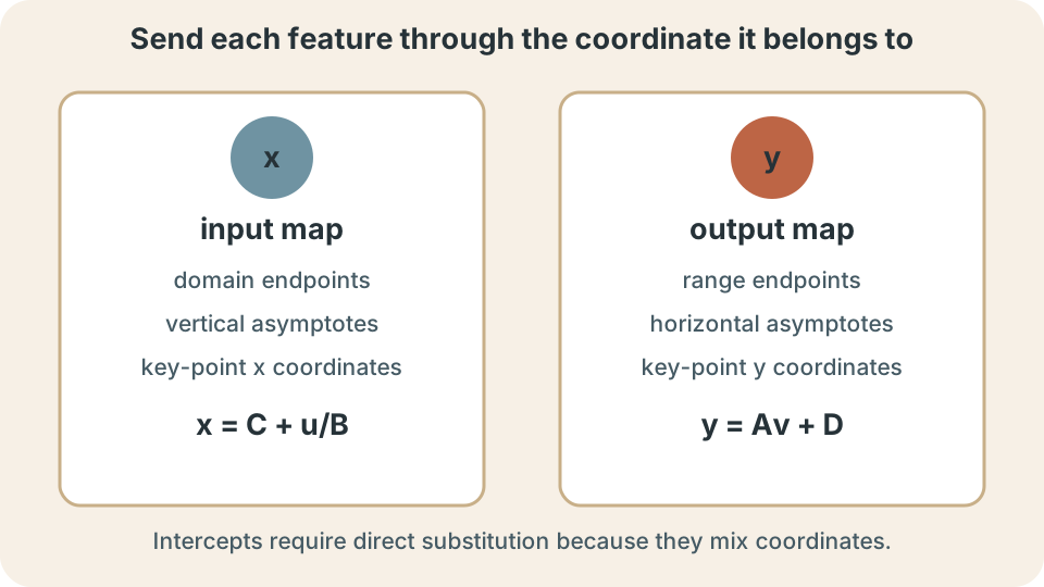
Derive or apply the point map $\left(u,v\right)\mapsto\left(C+\frac{u}{B},Av+D\right)$. Transform several key points. Map input restrictions and vertical asymptotes through the horizontal coordinate rule. Map range endpoints and horizontal asymptotes through the output rule. Calculate intercepts directly.

Check one mapped point by substitution. Verify reciprocal horizontal scale and reflection directions. Confirm domain and range with algebra. Attach units when parameters model physical quantities. Finish by describing the transformed function in words.

Practice and connection forward

Consider $g(x)=3f[-2(x+1)]-4$. Here $A=3$, $B=-2$, $C=-1$, and $D=-4$. The graph shifts left one, compresses horizontally by $\frac{1}{2}$, and reflects across the $y$ axis. It stretches vertically by three and shifts down four. Each effect follows from the signed map.

Map old point $(6,-1)$. Its new input is $-1+\frac{6}{-2}=-4$. Its new output is $3(-1)-4=-7$. Therefore the mapped point is $(-4,-7)$. Substitution into the general map verifies both coordinates.

Find the domain of $\sqrt{5-2x}$. Require $5-2x\geq0$, so $x\leq\frac{5}{2}$. Without looking back, derive why $f(Bx)$ uses reciprocal horizontal scale. Inverse functions will reverse input–output roles and reflect graphs across $y=x$. Later modeling will use transformations to interpret fitted parameters.