Trigonometric Graphs

Trigonometric graphs turn circular motion into a record of change. A point moving around a circle repeatedly produces horizontal and vertical coordinates that rise, fall, and repeat. Graphs of sine, cosine, and tangent preserve that geometric structure while making patterns easy to measure. Their transformations describe amplitude, timing, offsets, and phase in real systems. This lesson develops those ideas through construction, interpretation, and model checking.

Translate unit-circle motion into a graph

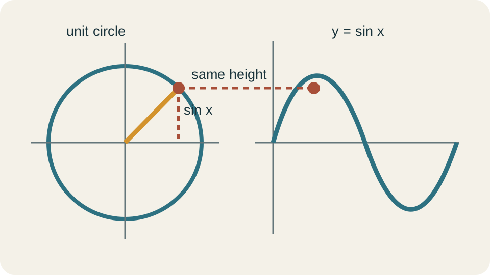
Place a point at angle $x$ on a unit circle, where $x$ is measured counterclockwise from the positive horizontal axis. The point has coordinates $(\cos x,\sin x)$. The first coordinate measures horizontal position, and the second measures vertical position. A graph of $y=\sin x$ records the vertical coordinate against the accumulated angle. A graph of $y=\cos x$ records the horizontal coordinate against that same angle.

At $x=0$, the point is $(1,0)$, so sine begins at zero while cosine begins at one. At $x=\dfrac{\pi}{2}$, the point is $(0,1)$, so sine reaches one and cosine reaches zero. At $x=\pi$, the point is $(-1,0)$. At $x=\dfrac{3\pi}{2}$, it is $(0,-1)$. At $x=2\pi$, the point returns to $(1,0)$ and the coordinate cycle repeats.

This correspondence explains the smooth wave shape without relying on a memorized sketch. Small changes in angle cause small changes in position, so the curves have no jumps. The vertical and horizontal coordinates remain between negative one and one. Their values repeat whenever the angle increases by one full rotation. Circular geometry therefore determines range, continuity, and periodicity together.

Read the parent sine graph

The parent function $y=\sin x$ has domain $\mathbb R$, meaning every real number may be used as an input. Its range is $[-1,1]$, so its output never falls below negative one or rises above one. The square brackets include both endpoints. The function crosses the horizontal axis at integer multiples of $\pi$. These zeros occur because the unit-circle point lies on the horizontal axis.

One basic cycle can be tracked through five key points: $(0,0)$, $\left(\dfrac{\pi}{2},1\right)$, $(\pi,0)$, $\left(\dfrac{3\pi}{2},-1\right)$, and $(2\pi,0)$. The graph rises from the midline to a maximum, returns to the midline, falls to a minimum, and returns again. Equal input intervals of $\dfrac{\pi}{2}$ separate these landmarks. Smooth connection between them reflects continuous rotation. Repeating the pattern extends the graph in both directions.

Sine is an odd function because $\sin(-x)=-\sin x$. Geometrically, reversing the angle reflects the unit-circle point across the horizontal axis. Graphically, rotating the sine curve by $180^\circ$ about the origin leaves it unchanged. This origin symmetry is a useful error check. A proposed sine graph lacking that symmetry cannot be the untransformed parent function.

Read the parent cosine graph

The parent function $y=\cos x$ also has domain $\mathbb R$ and range $[-1,1]$. Its key points are $(0,1)$, $\left(\dfrac{\pi}{2},0\right)$, $(\pi,-1)$, $\left(\dfrac{3\pi}{2},0\right)$, and $(2\pi,1)$. Cosine begins at a maximum because it records the unit-circle point’s horizontal coordinate. The curve descends through the midline, reaches a minimum, and returns. Its cycle has the same length as sine’s cycle.

Cosine is an even function because $\cos(-x)=\cos x$. Reversing the angle reflects a unit-circle point across the horizontal axis but leaves its horizontal coordinate unchanged. The graph is therefore symmetric about the vertical axis. Values at opposite inputs agree. This symmetry provides another fast check on a sketch or table.

Sine and cosine differ by a horizontal shift rather than by shape. The identity $\sin x=\cos\left(x-\dfrac{\pi}{2}\right)$ shifts cosine right by $\dfrac{\pi}{2}$. Equivalently, $\cos x=\sin\left(x+\dfrac{\pi}{2}\right)$. These formulas show that the two coordinates trace the same oscillation one quarter-cycle apart. Phase relationships like this are central in wave and circuit models.

Define period and periodicity

A function is periodic if some positive number $P$ satisfies $f(x+P)=f(x)$ for every input in the domain. The smallest positive such number is the fundamental period. Sine and cosine have fundamental period $2\pi$. One full angle increase of $2\pi$ returns the unit-circle point to its starting position. The graph then repeats the same outputs in the same order.

Period measures input spacing, not vertical size. If the horizontal axis represents time, period has units of time. If it represents distance, period has units of length. If it represents a dimensionless angle in radians, period is written as $2\pi$. Attaching the correct interpretation to the horizontal axis prevents an abstract number from being mistaken for a physical duration.

Frequency counts cycles per unit input and is reciprocal to period. When the input is time, $f=\dfrac{1}{T}$, where $T$ is the period. The symbol $f$ conventionally represents frequency, while $T$ conventionally represents one-cycle duration. If $T=0.250\,\mathrm{s}$, then $f=4.00\,\mathrm{Hz}$, where one hertz equals one cycle per second. Period and frequency describe the same repetition from complementary viewpoints.

Interpret amplitude and midline

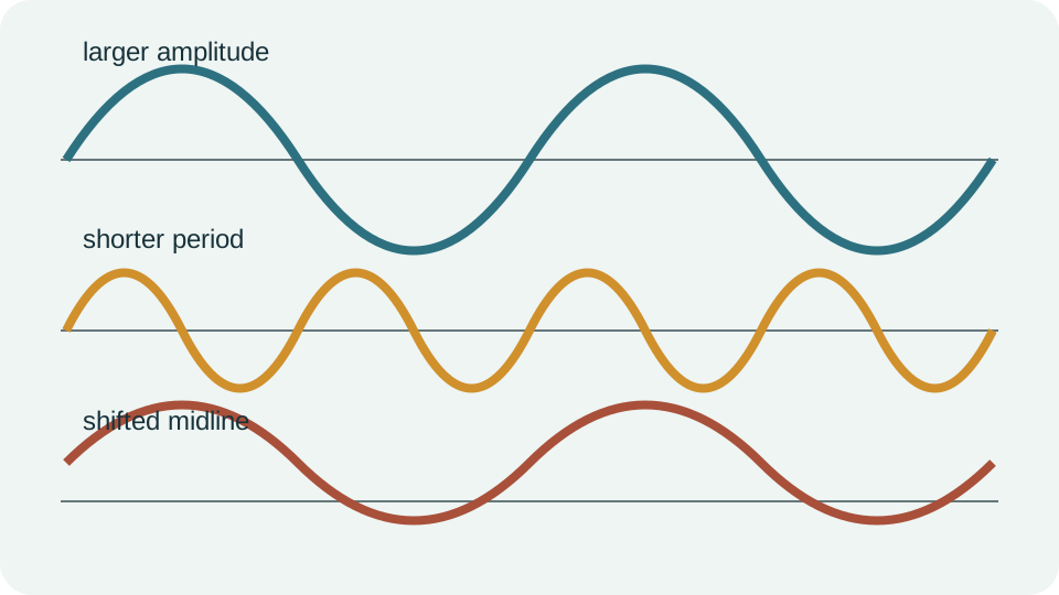
For $y=A\sin x+D$ or $y=A\cos x+D$, the amplitude is $|A|$. Absolute-value bars make amplitude nonnegative because amplitude measures distance from the midline. The midline is the horizontal line $y=D$. The maximum is $D+|A|$, and the minimum is $D-|A|$. Half the difference between maximum and minimum recovers amplitude.

Specifically, $|A|=\dfrac{y_{\max}-y_{\min}}{2}$ and $D=\dfrac{y_{\max}+y_{\min}}{2}$. The first formula takes half the total vertical span. The second averages the extremes to locate their center. Both formulas use a horizontal fraction bar to group the full numerator. These relationships allow model parameters to be read directly from data.

A negative coefficient reflects the graph across its midline. For example, $y=-3\cos x+5$ has amplitude three and midline $y=5$. It begins at the minimum value two rather than the maximum value eight. The negative sign controls orientation, not amplitude magnitude. Calling negative three the amplitude confuses signed transformation with geometric distance.

Derive the transformed period

Consider $y=A\sin[B(x-C)]+D$. The quantity inside the sine brackets is the function’s angle or phase. One sine cycle occurs when that phase changes by $2\pi$. If $x$ changes by $P$, the phase changes in magnitude by $|B|P$. Setting $|B|P=2\pi$ gives $P=\dfrac{2\pi}{|B|}$.

The coefficient $B$ is therefore not itself the period. A larger magnitude of $B$ makes the phase advance faster and compresses the graph horizontally. For $B=2$, the period is $\pi$, so two cycles fit into an interval of length $2\pi$. For $B=\dfrac{1}{3}$, the period is $6\pi$, so the graph stretches horizontally. Reciprocal reasoning explains the transformation better than a memorized formula alone.

When the horizontal input has physical units, the sine argument must be dimensionless. In $y=A\sin(\omega t)+D$, angular frequency $\omega$ has units of radians per second and $t$ has units of seconds. Their product is an angle in radians, which is dimensionless in dimensional analysis. The period is $T=\dfrac{2\pi}{|\omega|}$. Units reduce to seconds because dividing by inverse seconds produces seconds.

Interpret phase shift correctly

In factored form $y=A\sin[B(x-C)]+D$, the phase shift is $C$. Positive $C$ shifts the parent graph right, while negative $C$ shifts it left. The subtraction appears inside the input, so its visible sign acts opposite to the direction of the graph’s translation. This is the same input-transformation rule used for other functions. A marked key point moves from $x=0$ to $x=C$.

Expanded expressions should be factored before the shift is read. For example, $\sin(2x-\pi)$ becomes $\sin\left[2\left(x-\dfrac{\pi}{2}\right)\right]$. The phase shift is therefore $\dfrac{\pi}{2}$ to the right, not $\pi$. The coefficient two multiplies the entire shifted input. Ignoring that grouping is a common source of incorrect graphs.

Phase shift is not always unique because the function is periodic. A right shift of $\dfrac{\pi}{2}$ for sine can be represented by other shifts differing by integer multiples of $2\pi$. Different sine and cosine forms may model the same curve. A useful phase choice aligns a recognizable event, such as a maximum or upward midline crossing, with the data. Equivalent representations should be judged by their outputs rather than by superficial parameter differences.

Construct a sine or cosine graph systematically

Begin by identifying amplitude, midline, period, and phase shift. Draw the midline first because the oscillation is organized around it. Mark an interval of one complete period beginning at a convenient phase reference. Divide that interval into four equal subintervals. These quarter-period locations correspond to the five key stages of a sine or cosine cycle.

For positive sine, the sequence is midline rising, maximum, midline falling, minimum, and midline rising again. For positive cosine, it is maximum, midline falling, minimum, midline rising, and maximum. A negative coefficient reverses highs and lows around the midline. Plot the five points before drawing a smooth curve. Then repeat the pattern one period left and right.

Consider $y=-2\sin\left(\dfrac{x}{3}\right)+1$. Its amplitude is two, midline is $y=1$, and period is $\dfrac{2\pi}{1/3}=6\pi$. With no phase shift, quarter-period spacing is $\dfrac{3\pi}{2}$. The negative coefficient makes the graph begin at the midline and move downward. Its maximum is three and its minimum is negative one.

Model periodic height from physical data

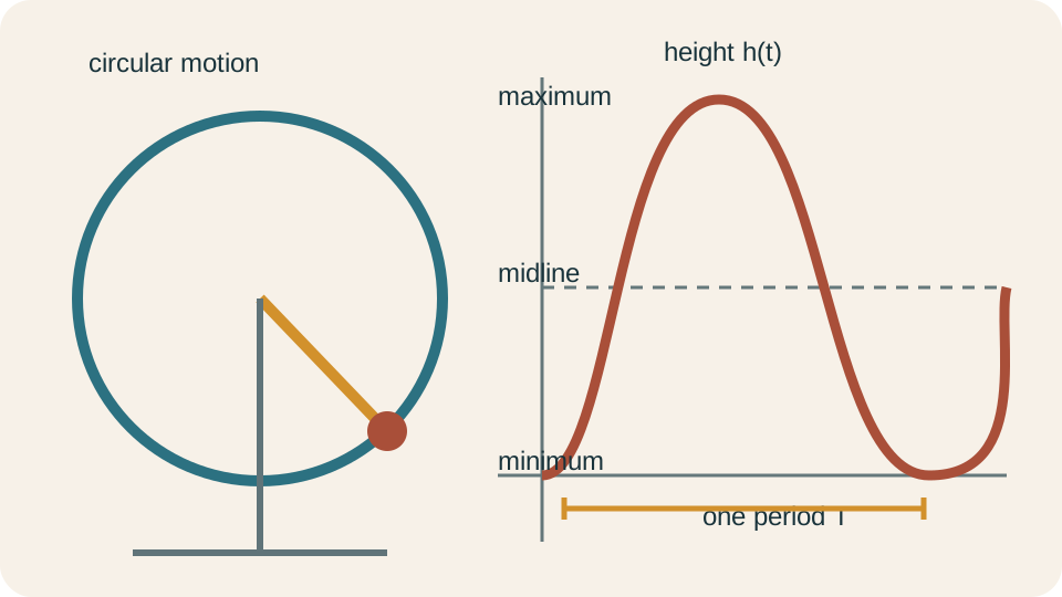
A wheel seat moves between $2.0\,\mathrm{m}$ and $18.0\,\mathrm{m}$ and completes a revolution every $40.0\,\mathrm{s}$. Its amplitude is $\dfrac{18.0\,\mathrm{m}-2.0\,\mathrm{m}}{2}=8.0\,\mathrm{m}$. Its midline is $\dfrac{18.0\,\mathrm{m}+2.0\,\mathrm{m}}{2}=10.0\,\mathrm{m}$. The vertical units remain meters throughout these calculations. The period is supplied as $40.0\,\mathrm{s}$.

Suppose the seat begins at its lowest point when $t=0$. A convenient model is $h(t)=10.0\,\mathrm{m}-(8.0\,\mathrm{m})\cos\left(\dfrac{2\pi t}{40.0\,\mathrm{s}}\right)$. The negative cosine begins below the midline because $\cos0=1$. At $t=0$, the model gives $h(0)=2.0\,\mathrm{m}$. At half a period, $t=20.0\,\mathrm{s}$, it gives the maximum $18.0\,\mathrm{m}$.

The cosine argument is dimensionless because $t$ and $40.0\,\mathrm{s}$ carry the same time units. The quotient $t/(40.0\,\mathrm{s})$ counts fractions of a revolution. Multiplication by $2\pi$ converts that fraction into angular phase. Every parameter has an interpretable role rather than serving as a curve-fitting decoration. Checking endpoints and quarter-period events confirms that the formula matches the stated motion.

Analyze the tangent graph

Tangent is defined by $\tan x=\dfrac{\sin x}{\cos x}$. It equals zero where sine is zero and cosine is nonzero, so zeros occur at $x=k\pi$ for integers $k$. It is undefined where cosine is zero, at $x=\dfrac{\pi}{2}+k\pi$. Near those inputs, the quotient grows without bound in positive or negative directions. The graph has vertical asymptotes at those excluded values.

An asymptote is a line the graph approaches without taking a finite value there. It is not a removable hole and should not be drawn as part of the function. Between consecutive asymptotes, the parent tangent graph increases from negative infinity to positive infinity. Its fundamental period is $\pi$, not $2\pi$. The quotient repeats after half a full rotation because both sine and cosine change sign, leaving their ratio unchanged.

For $y=A\tan[B(x-C)]+D$, the period is $\dfrac{\pi}{|B|}$. Tangent has no amplitude because its outputs are unbounded. The coefficient $A$ changes vertical steepness and may reflect the branches, but it does not bound their height. The line $y=D$ is a centerline rather than a midline between finite extrema. Applying sine vocabulary mechanically to tangent obscures these structural differences.

Read information from a graph

To estimate a sinusoid’s period, measure the horizontal distance between consecutive matching landmarks. Maxima to maxima, minima to minima, or upward midline crossings to upward midline crossings all work. Using a maximum to the next minimum measures half a period. The direction of crossing matters because adjacent midline crossings are also half a period apart. Consistent landmark choice prevents a factor-of-two error.

Amplitude is the vertical distance from the midline to an extreme. It is not the full peak-to-trough range. The midline can be found by averaging maximum and minimum values. A phase reference then comes from locating a maximum, minimum, or directional crossing. Reading all four features before selecting sine or cosine makes model construction deliberate.

Graphs also reveal whether a proposed model is plausible. A periodic model should repeat with stable timing if its parameters are constant. Measured peaks outside the predicted range may indicate noise, changing amplitude, or an inappropriate model. Drift in peak spacing may indicate changing frequency. Interpretation includes recognizing when a simple sinusoid is insufficient.

Use technology without surrendering reasoning

Graphing software can display a function quickly, but its viewing window controls what is visible. A narrow window may hide a full cycle, while a wide window may compress important structure. Automatic scaling can make different amplitudes appear similar. Entering degrees while the software expects radians changes the horizontal scale. A hand prediction should guide window selection before the graph is trusted.

Tables provide numerical checks at key inputs. Evaluate the model at the start, quarter period, half period, three-quarter period, and full period. These five values should match the expected cycle sequence. Exact values are preferable when special angles are involved. Decimal sampling supplements rather than replaces structural analysis.

Regression can estimate sinusoidal parameters from noisy data, but a fitted curve is not automatically a meaningful mechanism. Units, residual patterns, and measurement context still matter. The fitted period should agree with observed repetition, and the amplitude should match vertical variation. A graph is evidence to interpret, not a verdict produced by software. Mathematical judgment remains necessary after computation.

Diagnose common graphing errors

One common error is labeling $D$ as amplitude. The parameter $D$ locates the midline, while $|A|$ gives the distance from that line to an extreme. Another error is using $B$ as the period instead of calculating a reciprocal relationship. A third is reading a phase shift before factoring the inner coefficient. Each mistake can be prevented by translating parameters into geometric questions.

Another error is plotting isolated key points with straight segments. Sine and cosine curves are smooth because circular motion changes smoothly. Sharp corners misrepresent their rates of change. Tangent branches must also stop at asymptotes rather than crossing them. Graph shape carries mathematical information beyond the locations of a few points.

Dimensional mistakes are especially important in applications. Adding a distance to a dimensionless sine value is invalid unless the sine is first multiplied by a distance amplitude. Putting a dimensional quantity alone inside sine is also invalid. The argument must reduce to a pure number, usually an angle in radians. Unit checks reveal model errors that a visually attractive graph may conceal.

Practice a complete construction routine

Analyze $y=-3\sin(2x)+5$. Its amplitude is three, its midline is $y=5$, and its period is $\dfrac{2\pi}{2}=\pi$. Its quarter-period spacing is $\dfrac{\pi}{4}$. The negative coefficient makes the graph move downward from the midline at $x=0$. Maximum and minimum values are eight and two.

Next consider $y=4\cos\left[\dfrac{1}{3}(x-\pi)\right]-1$. Its amplitude is four, midline is $y=-1$, and period is $6\pi$. Its phase shift is $\pi$ to the right. At $x=\pi$, the positive cosine begins at its maximum value three. The minimum value is negative five.

Finally, construct a tangent model with centerline $y=2$, period $\dfrac{\pi}{4}$, and central crossing at $x=1$. Since $\dfrac{\pi}{|B|}=\dfrac{\pi}{4}$, choose $B=4$. One model is $y=\tan[4(x-1)]+2$. Its neighboring asymptotes lie one half-period from the central crossing. Checking those geometric features verifies the parameters.

Consolidate periodic-graph reasoning

Trigonometric graphs are coordinate records of circular motion. Sine tracks vertical position, cosine tracks horizontal position, and tangent tracks their quotient. Period records horizontal repetition, amplitude records bounded vertical excursion, and phase locates a cycle relative to an origin. Midline and vertical shift locate the oscillation’s center. These meanings should be stated before equations are manipulated.

A reliable workflow moves from context to features and then to formula. Identify extrema and center, measure repetition, select a reference event, choose sine or cosine, and check key points. For tangent, locate asymptotes and central crossings instead of searching for amplitude. Units and dimensional arguments remain part of every physical model. Graphs and equations should confirm one another.

These skills prepare the way for trigonometric identities, wave mechanics, simple harmonic motion, and Fourier analysis. Later topics may combine many sinusoidal components or allow parameters to vary. The foundational questions remain the same: what repeats, how large is the variation, where is the center, and how is timing shifted? A graph makes those relationships visible. Sound interpretation turns that picture into quantitative understanding.