Systems and Phase Planes

Many evolving quantities interact, so one differential equation is often not enough. A system tracks several state variables at once and specifies how each rate depends on the whole state. A phase plane then shows the state as a moving point without using time as a plotted axis. This geometric view reveals equilibria, attraction, repulsion, oscillation, and transition paths even when formulas are difficult to obtain. The goal of this lesson is to connect equations, vectors, trajectories, and stability as four descriptions of the same dynamics.

Learning objectives and state-space thinking

By the end of this lesson, you will convert a higher-order equation into a first-order system, interpret a vector field, and locate equilibria. You will solve two-dimensional linear systems by eigenmodes and classify common equilibrium types. You will use nullclines to sketch nonlinear motion and a Jacobian matrix to analyze behavior near an equilibrium. You will also distinguish what a phase portrait proves from what it merely suggests. These objectives build a workflow for qualitative reasoning rather than a list of pictures to memorize.

A state is the minimum collection of variables needed to predict future evolution once a model and an initial state are specified. For a moving mass, position alone is insufficient because the same position with different velocity leads to different futures. The pair $(x,v)$ can supply the needed state, where $x$ is position and $v$ is velocity. In a two-species population model, the state might instead be $(x,y)$, with each coordinate representing a population. A state space contains every allowed combination of those variables.

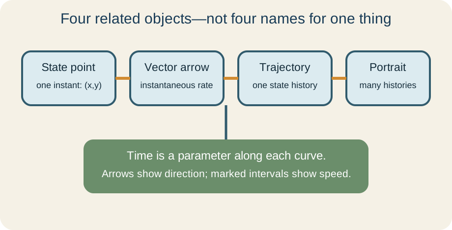
The phase plane is a two-dimensional state space. A point represents an instantaneous state, while a curve represents a sequence of states followed over time. The independent variable $t$ is still present in the functions $x(t)$ and $y(t)$, but it is not one of the plotted axes. Arrows along trajectories indicate increasing time. The overview below separates the objects that students often accidentally treat as interchangeable.

Convert higher-order equations to first-order systems

Every ordinary differential equation of order $n$ can be represented as a system of $n$ first-order equations under standard smoothness assumptions. Consider $x''+ax'+bx=0$, where primes mean derivatives with respect to time. Define $v=x'$, so $v$ records velocity when $x$ is position. Then $x'=v$ and $v'=x''=-bx-av$. The second-order equation has become a first-order system in the state $(x,v)$ without changing its solutions.

The conversion works because the new variables preserve all derivative information needed by the original equation. For a third-order equation, one could define $x_1=x$, $x_2=x'$, and $x_3=x''$. The resulting chain begins with $x_1'=x_2$ and $x_2'=x_3$, while the original equation determines $x_3'$. Initial values for the first-order system correspond exactly to the initial position and derivatives of the higher-order problem. This equivalence lets one general theory and one family of numerical methods handle equations of many orders.

Units provide an important check. If $x$ is measured in meters and $t$ in seconds, then $v=x'$ has units of meters per second and $v'$ has units of meters per second squared. In $x''+ax'+bx=0$, the coefficient $a$ must have units of inverse seconds and $b$ must have units of inverse seconds squared. Terms can be added only when their units agree. A phase plane may therefore place quantities with different units on its two axes, which is entirely valid when each axis is labeled.

Read an autonomous vector field

An autonomous system has the form $\mathbf{x}'=\mathbf{f}(\mathbf{x})$, meaning its rule does not depend explicitly on time. Bold $\mathbf{x}$ denotes a state vector rather than a single number. At each state, $\mathbf{f}(\mathbf{x})$ gives the instantaneous velocity through state space. Its direction indicates where the state moves next, and its magnitude indicates how quickly it moves with respect to time. Drawing representative arrows creates a direction field in the phase plane.

For $x'=y$ and $y'=-x$, evaluate the field at several points. At $(1,0)$, the vector is $(0,-1)$, so motion is initially downward. At $(0,1)$, the vector is $(1,0)$, so motion is initially rightward. At $(-1,0)$, the vector is $(0,1)$, and at $(0,-1)$ it is $(-1,0)$. Together these directions indicate clockwise circulation around the origin.

A trajectory must be tangent to the vector field at every point it visits. Two distinct solution trajectories cannot cross at an ordinary point when the system has unique solutions, because crossing would assign two futures to the same state. Arrow length depends on plotting conventions, so compare speeds only when the diagram uses a consistent scale. A geometric curve without arrows does not reveal the direction of time. A portrait without time markers also cannot show speed directly.

Find equilibria and define stability

An equilibrium $\mathbf{x}_*$ satisfies $\mathbf{f}(\mathbf{x}_*)=\mathbf{0}$. The star labels a particular state, and the zero vector means every component derivative is zero. A solution starting exactly there remains constant for all time. For the system $x'=x-y$ and $y'=x+y-2$, solve $x-y=0$ and $x+y-2=0$. The unique equilibrium is $(1,1)$.

Stability describes how nearby solutions behave, not merely what happens at the exact equilibrium. An equilibrium is stable in the sense of Lyapunov if states starting sufficiently close remain close for all future time. It is asymptotically stable if it is stable and nearby states also approach it as $t$ increases. An unstable equilibrium has arbitrarily nearby initial states that eventually leave a chosen neighborhood. These definitions distinguish neutral persistence from genuine attraction.

A marble in a bowl provides a useful analogy for asymptotic stability when friction removes energy. A marble balanced on top of a hill illustrates instability because a tiny displacement grows. A frictionless marble in an ideal bowl can orbit without approaching the bottom, suggesting stability without asymptotic attraction. Analogies guide intuition but do not replace definitions. Mathematical classification must follow from the system’s local or global behavior.

Solve linear systems with eigenmodes

For a linear autonomous system $\mathbf{x}'=A\mathbf{x}$, the matrix $A$ maps the current state to its instantaneous rate. Suppose $A\mathbf{v}=\lambda\mathbf{v}$, where $\mathbf{v}$ is an eigenvector and $\lambda$ its eigenvalue. Then $\mathbf{x}(t)=e^{\lambda t}\mathbf{v}$ is a solution because differentiating multiplies it by $\lambda$. The eigenvector gives an invariant direction, while the eigenvalue controls growth, decay, or rotation along the corresponding mode. Two independent eigenvectors usually provide a basis for all initial states in two dimensions.

Consider $A=\begin{bmatrix}1&0\\0&-2\end{bmatrix}$ with entries measured in inverse seconds. Its eigenvectors are the coordinate directions, with eigenvalues $1\,\mathrm{s}^{-1}$ and $-2\,\mathrm{s}^{-1}$. The general solution is $\mathbf{x}(t)=C_1e^{t/(1\,\mathrm{s})}\mathbf{v}_1+C_2e^{-2t/(1\,\mathrm{s})}\mathbf{v}_2$. The first mode grows as time increases, while the second decays. Therefore most states eventually depart along the first coordinate direction.

The constants $C_1$ and $C_2$ encode the initial condition. At $t=0$, both exponential factors equal one, so $\mathbf{x}(0)=C_1\mathbf{v}_1+C_2\mathbf{v}_2$. Decomposing the initial state into eigenvector components determines the constants. If an initial state lies exactly on a decaying eigenvector, it can approach an otherwise unstable equilibrium. Stability classification nevertheless concerns all sufficiently nearby states, so one exceptional path does not make the equilibrium stable.

Classify two-dimensional linear equilibria

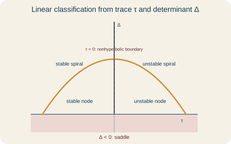
Two negative real eigenvalues produce a stable node, while two positive real eigenvalues produce an unstable node. Real eigenvalues with opposite signs produce a saddle, which is always unstable. At a node, trajectories generally approach or leave tangent to a dominant eigenvector. At a saddle, one eigendirection is stable and the other is unstable. The determinant and trace of $A$ can summarize these cases because their values equal the eigenvalue product and sum.

A complex conjugate pair has the form $\lambda=\alpha\pm i\beta$, where $i^2=-1$. The real part $\alpha$ controls exponential growth or decay, while the nonzero imaginary part $\beta$ produces rotation. Negative $\alpha$ gives a stable spiral, and positive $\alpha$ gives an unstable spiral. When $\alpha=0$ in a linear system, closed curves may form a center. Rotation direction must be found from the vector field rather than from eigenvalues alone.

Repeated eigenvalues require attention to the number of independent eigenvectors. Two independent eigenvectors can produce a star node, while one eigenvector creates a defective or improper node with generalized-eigenvector behavior. A zero eigenvalue or a purely imaginary pair is nonhyperbolic because at least one eigenvalue has zero real part. For nonlinear systems, such cases are often inconclusive under first-order linearization. The classification chart below organizes the hyperbolic cases and flags the boundary where more analysis is needed.

Use nullclines for nonlinear systems

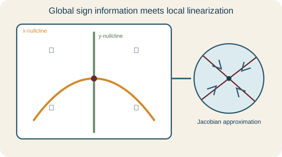
For $x'=f(x,y)$ and $y'=g(x,y)$, the curve $f(x,y)=0$ is the $x$-nullcline. Along it, horizontal motion temporarily stops because $x'=0$, so field arrows are vertical unless both derivatives vanish. The curve $g(x,y)=0$ is the $y$-nullcline, where vertical motion stops and arrows are horizontal. Intersections of the two nullclines are equilibrium candidates. Substitution confirms which intersections lie in the permitted domain.

Nullclines divide the plane into regions where the signs of $x'$ and $y'$ are often constant. If $x'>0$, arrows point to the right, and if $x'<0$, they point to the left. Likewise, $y'>0$ means upward motion and $y'<0$ means downward motion. Combining the two signs gives northeast, northwest, southeast, or southwest motion. Sampling one point in each region can therefore organize a qualitative sketch efficiently.

Consider the competition model $x'=x(1-x-y)$ and $y'=y(1-\frac{x}{2}-y)$. The $x$-nullclines are $x=0$ and $1-x-y=0$, while the $y$-nullclines are $y=0$ and $1-\frac{x}{2}-y=0$. Their intersections identify boundary and interior equilibrium candidates. The factors $x$ and $y$ also show that the coordinate axes are invariant, so nonnegative populations cannot cross an axis under unique solutions. A sign chart then predicts which populations increase or decrease in each biologically relevant region.

Linearize near a nonlinear equilibrium

Near an equilibrium $\mathbf{x}_*$, write the displacement as $\mathbf{u}=\mathbf{x}-\mathbf{x}_*$. A differentiable nonlinear system has the local approximation $\mathbf{u}'=J(\mathbf{x}_*)\mathbf{u}$ plus higher-order terms. The Jacobian $J$ is the matrix of first partial derivatives of the component functions. Each entry measures how one rate changes when one state variable changes. Evaluating at the equilibrium produces the best first-order linear model there.

For $x'=x-x^2-xy$ and $y'=2y-xy-y^2$, the Jacobian is $J(x,y)=\begin{bmatrix}1-2x-y&-x\\-y&2-x-2y\end{bmatrix}$. At any equilibrium, substitute its coordinates into this matrix before finding eigenvalues. If every eigenvalue has nonzero real part, the equilibrium is hyperbolic. A hyperbolic sink, source, or saddle has the same local qualitative type as its linearization. The portrait may bend away from the equilibrium, but local attraction and repulsion persist.

If an eigenvalue has zero real part, first-order terms do not settle the competition between growth and decay. For example, $x'=-x^3$ has linearization $x'=0$ at the origin, yet the nonlinear origin is asymptotically stable. By contrast, $x'=x^3$ has the same linearization but an unstable origin. Higher-order terms distinguish the two systems. In a nonhyperbolic case, use another argument such as a Lyapunov function, invariant set, normal form, or direct sign analysis.

Build and check a phase portrait

Begin by finding equilibria and all nullclines. Next determine arrow directions on nullclines and signs in the regions they create. Linearize at each equilibrium when appropriate, then draw local eigendirections or spiral orientation. Connect the local information with trajectories that remain tangent to the field and do not cross. Finally, label axes, equilibrium types, invariant sets, and the direction of increasing time.

Do not confuse a trajectory’s shape with its speed. Two systems can trace the same geometric curves at different rates because multiplying a vector field by a positive scalar function changes timing without reversing paths. Closely spaced time markers indicate slower motion, while widely spaced markers indicate faster motion. Standard phase portraits often omit such markers, so speed cannot be inferred from curve density alone. Arrow magnitude in a software plot is meaningful only if the plotting routine has not normalized every vector.

Check the portrait against algebraic invariants. A trajectory should never cross a uniqueness-preserving invariant axis, and its tangent must agree with the local vector. A claimed stable equilibrium must not have arrows pointing away along any nearby direction. A periodic orbit cannot pass through an equilibrium because motion there stops. Numerical simulations can test a sketch, but they should sample several initial states and step sizes rather than serve as the sole proof.

Guided analysis and practice

Convert $x''+5x'+6x=0$ by defining $v=x'$. The system is $x'=v$ and $v'=-6x-5v$. Its matrix is $A=\begin{bmatrix}0&1\\-6&-5\end{bmatrix}$, whose characteristic equation is $\lambda^2+5\lambda+6=0$. The eigenvalues are $-2\,\mathrm{s}^{-1}$ and $-3\,\mathrm{s}^{-1}$ when time is measured in seconds. Both are negative and real, so the origin is a stable node.

Now classify a system whose eigenvalues are $2\,\mathrm{s}^{-1}$ and $-3\,\mathrm{s}^{-1}$. Their opposite signs imply one growing and one decaying eigendirection. The origin is a saddle and therefore unstable, even though an initial state exactly on the stable eigendirection approaches it. Sketch two invariant eigenvector lines and orient their arrows according to the eigenvalue signs. Fill neighboring trajectories so they approach along the stable direction and depart along the unstable direction.

For independent practice, analyze $x'=y$ and $y'=x(1-x^2)-0.4y$, with time in seconds and consistently scaled state units. Find the equilibria, compute the Jacobian at each one, and classify every hyperbolic equilibrium. Then identify where $x'=0$ and $y'=0$, use signs to orient the field, and sketch plausible connecting trajectories. Check that every drawn trajectory is tangent to the local vector field. Explain which conclusions follow from local eigenvalues and which require broader phase-plane evidence.

Synthesis and connection forward

A system of differential equations is a rule for motion through state space. The vector field supplies local direction and speed, while trajectories integrate that local information into histories. Equilibria are stationary states, and stability asks how neighboring histories respond. Eigenvalues make these questions tractable for linear systems. Nullclines and Jacobians extend much of the same reasoning to nonlinear systems.

The most reliable workflow moves repeatedly between representations. Translate a physical or biological model into equations, evaluate its vector field, locate special sets, classify local behavior, and compare the portrait with the original context. Explain every symbol as it enters the model, including state coordinates, derivatives, matrix entries, and eigenvalues. Preserve units when the variables are dimensional. Use computation to explore but use mathematical structure to justify conclusions.

Phase-plane reasoning leads naturally to bifurcations, nonlinear oscillations, control theory, and numerical simulation. In those subjects, parameters may move equilibria or change their stability. Closed orbits can represent sustained oscillations, while stable and unstable manifolds organize transport through the state space. The foundational ideas remain the same: a state, a rate rule, and the geometry generated by their interaction. Mastering that connection is more durable than memorizing any single portrait.