Eigenvalues and Eigenvectors

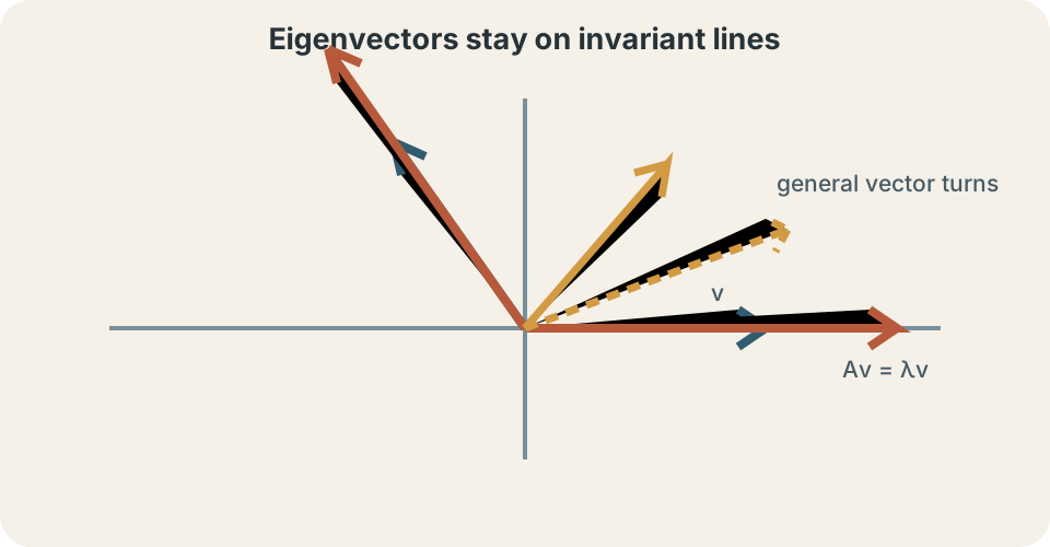
A linear transformation usually changes both a vector’s magnitude and its direction. Some exceptional directions do not turn away from their own line. Vectors on those directions are only scaled, possibly with a sign reversal. These are eigenvector directions, and their scale factors are eigenvalues. They reveal a transformation’s simplest internal actions.

Eigenstructure matters because complicated behavior can be decomposed into simple modes. Repeated matrix multiplication becomes repeated scalar multiplication along eigenvectors. Systems of differential equations separate into exponential modes when enough eigenvectors exist. Vibrations, population models, stability, and data analysis all use this idea. The same definition connects them.

This lesson begins geometrically and derives the characteristic equation from the need for nonzero solutions. It then develops eigenspaces, multiplicity, diagonalization, powers, continuous dynamics, complex eigenvalues, and numerical verification. Every determinant and vector symbol will be interpreted. Worked examples preserve exact fractions. The goal is structural understanding rather than a determinant-only recipe.

Learning goals and an opening geometric question

You should identify eigenvectors as invariant directions and eigenvalues as scale factors. You should calculate eigenvalues and bases for eigenspaces. You should distinguish algebraic from geometric multiplicity. You should determine when a matrix is diagonalizable. You should interpret eigenstructure in repeated and continuous dynamics.

Imagine stretching a rubber sheet twice as much horizontally while leaving vertical distances unchanged. A horizontal arrow remains horizontal and doubles. A vertical arrow remains vertical and keeps its length. Most diagonal arrows change direction because their horizontal and vertical parts scale differently. The coordinate axes are eigenvector directions.

Now add a rotation by ninety degrees. No nonzero real arrow stays on its original line. That real transformation has no real eigenvectors. Complex numbers can still encode its rotation. The field of scalars determines which eigenstructure is visible.

The defining equation

Let $A$ be a square matrix representing a linear transformation. A nonzero vector $\mathbf v$ is an eigenvector when $A\mathbf v=\lambda\mathbf v$. Greek letter $\lambda$, pronounced lambda, is the eigenvalue. The equation says applying $A$ has the same effect as multiplying $\mathbf v$ by scalar $\lambda$. Direction stays on the same line.

The zero vector is excluded. It satisfies $A\mathbf0=\lambda\mathbf0$ for every scalar $\lambda$. Because zero has no direction, including it would make the definition meaningless. Every eigenspace contains zero as a vector-space requirement. Zero is simply not called an eigenvector.

An eigenvalue belongs to a matrix, while an eigenvector belongs to an eigenvalue’s solution set. One eigenvalue can have infinitely many eigenvectors because every nonzero scalar multiple of one eigenvector remains an eigenvector. If $A\mathbf v=\lambda\mathbf v$, then $A(c\mathbf v)=cA\mathbf v=\lambda(c\mathbf v)$. The direction rather than one arrow length is fundamental. Scalar multiples describe that same invariant line.

What the eigenvalue does

If $\lambda>1$, the eigenvector keeps orientation and grows in magnitude. If $0<\lambda<1$, it keeps orientation and shrinks. If $\lambda=1$, every vector in that eigendirection is fixed. These statements describe one application. Repeated applications raise the factor to a power.

If $\lambda<0$, the transformed vector reverses orientation along the same line. Its magnitude is multiplied by $|\lambda|$. For $\lambda=-2$, the vector flips and doubles. Two applications multiply by $(-2)^2=4$, restoring orientation. Sign and magnitude carry distinct geometric information.

If $\lambda=0$, $A\mathbf v=\mathbf0$. The transformation collapses that nonzero direction into zero. Therefore $A$ is not invertible. A zero eigenvalue is equivalent to a nontrivial null space. This connects eigenvalues to singularity.

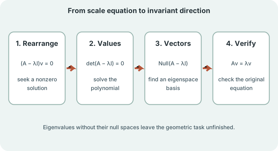
Rearranging creates a homogeneous system

Move the right side of $A\mathbf v=\lambda\mathbf v$ to the left. Because $\lambda\mathbf v=\lambda I\mathbf v$, the equation becomes $(A-\lambda I)\mathbf v=\mathbf0$. Matrix $I$ is the identity with ones on its main diagonal. Subtraction $A-\lambda I$ changes only those diagonal entries. The unknown remains vector $\mathbf v$.

We need a nonzero solution to this homogeneous system. An invertible coefficient matrix would have only the zero solution. Therefore $A-\lambda I$ must be singular. A square matrix is singular exactly when its determinant is zero. This produces the characteristic equation.

The equation is $\det(A-\lambda I)=0$. The determinant becomes a polynomial in $\lambda$. Its roots are eigenvalues. Different texts sometimes use $\det(\lambda I-A)$ instead. The roots agree even if the polynomial differs by an overall sign.

The characteristic polynomial

The characteristic polynomial is $p_A(\lambda)=\det(A-\lambda I)$ under one common convention. For an $n\times n$ matrix, it has degree $n$. The fundamental theorem of algebra guarantees $n$ complex roots when multiplicities are counted. Real matrices can have nonreal roots in conjugate pairs. Not every root must be distinct.

For a $2\times2$ matrix $A=\begin{bmatrix}a&b\\c&d\end{bmatrix}$, compute $p_A(\lambda)=(a-\lambda)(d-\lambda)-bc$. Expanding gives $\lambda^2-(a+d)\lambda+(ad-bc)$ under this convention. Quantity $a+d$ is the trace. Quantity $ad-bc$ is the determinant. Both are invariant under a change of basis.

Therefore the sum of two eigenvalues equals the trace and their product equals the determinant, counting multiplicity. These relationships provide checks. A zero determinant forces at least one zero eigenvalue. A negative determinant for a real $2\times2$ matrix forces real eigenvalues with opposite signs. These checks can reveal a sign error in the characteristic polynomial.

Worked eigenvalue calculation

Consider $A=\begin{bmatrix}3&1\\0&2\end{bmatrix}$. Subtract $\lambda I$ to obtain $\begin{bmatrix}3-\lambda&1\\0&2-\lambda\end{bmatrix}$. Its determinant is $(3-\lambda)(2-\lambda)$. Set this product equal to zero. The eigenvalues are $\lambda=3$ and $\lambda=2$.

The matrix is triangular, so its eigenvalues equal its diagonal entries. This is a theorem for every triangular matrix. The determinant calculation confirms it. Trace is $3+2=5$, matching $3+2$. Determinant is $6$, matching $(3)(2)$.

Finding eigenvalues is only the first half. Each value must be substituted into $(A-\lambda I)\mathbf v=\mathbf0$. The resulting null space gives its eigenspace. Do not solve the characteristic equation and stop. Directions carry the geometry.

Eigenspaces are null spaces

For eigenvalue $\lambda$, the eigenspace is $E_\lambda=\operatorname{Null}(A-\lambda I)$. It contains zero and every eigenvector associated with $\lambda$. The term “eigenvector” excludes zero, while “eigenspace” includes it. A basis gives independent directions spanning all associated eigenvectors. Null-space methods find that basis.

For $\lambda=3$ in the example, $A-3I=\begin{bmatrix}0&1\\0&-1\end{bmatrix}$. Equations require $y=0$, while $x$ is free. Thus $\mathbf v=t\begin{bmatrix}1\\0\end{bmatrix}$. A basis is $\left\{\begin{bmatrix}1\\0\end{bmatrix}\right\}$. Nonzero choices of parameter $t$ are eigenvectors.

For $\lambda=2$, $A-2I=\begin{bmatrix}1&1\\0&0\end{bmatrix}$. The equation is $x+y=0$, so $x=-y$. Write $\mathbf v=t\begin{bmatrix}-1\\1\end{bmatrix}$. The eigenspace basis is $\left\{\begin{bmatrix}-1\\1\end{bmatrix}\right\}$. This line differs from the first eigenspace.

Verification should be direct

Every proposed eigenpair should be checked in the original equation. For $\lambda=3$ and $\mathbf v=\begin{bmatrix}1\\0\end{bmatrix}$, multiplication gives $A\mathbf v=\begin{bmatrix}3\\0\end{bmatrix}=3\mathbf v$. The equality verifies both value and vector. A null-space arithmetic error would fail this test. Direct verification is faster than repeating the determinant calculation.

For $\lambda=2$ and $\mathbf v=\begin{bmatrix}-1\\1\end{bmatrix}$, multiplication gives $\begin{bmatrix}-2\\2\end{bmatrix}=2\begin{bmatrix}-1\\1\end{bmatrix}$. The transformed arrow remains on the same line. Its orientation is preserved because two is positive. Its length doubles. The geometric statement and algebraic equality agree.

An approximate numerical eigenpair can be checked with residual $\mathbf r=A\mathbf v-\lambda\mathbf v$. A small residual relative to relevant matrix and vector scales supports the approximation. A raw residual size without scale can be misleading. Exact examples should produce the zero vector. Numerical reporting should include a tolerance or relative residual.

Eigenvectors for distinct eigenvalues are independent

Eigenvectors associated with distinct eigenvalues are linearly independent. For a $2\times2$ matrix, two distinct eigenvalues therefore provide two independent eigenvector directions. Those vectors form a basis of the plane. Every vector can be written uniquely as their linear combination. This enables diagonalization.

The independence theorem extends to any finite collection of distinct eigenvalues. It does not say eigenvectors from the same eigenspace are automatically independent. Within one eigenspace, choose a basis. Scalar multiples do not add new directions. Dimension counts independent vectors.

A matrix with $n$ distinct eigenvalues is diagonalizable over a field containing those eigenvalues. Distinctness is sufficient but not necessary. Repeated eigenvalues can still supply enough eigenvectors. The total number of independent eigenvectors decides. Exactly $n$ independent directions are required in $n$ dimensions.

Algebraic and geometric multiplicity

Algebraic multiplicity counts how many times an eigenvalue appears as a root of the characteristic polynomial. Geometric multiplicity is the dimension of its eigenspace. The geometric multiplicity is at least one for an eigenvalue. It cannot exceed algebraic multiplicity. Their difference detects missing eigenvectors.

Identity matrix $I_2$ has characteristic polynomial $(1-\lambda)^2$. Eigenvalue one has algebraic multiplicity two. Its eigenspace is the entire plane because $(I_2-I_2)\mathbf v=\mathbf0$ for every vector. Geometric multiplicity is also two. The matrix is diagonalizable.

Matrix $J=\begin{bmatrix}1&1\\0&1\end{bmatrix}$ has the same repeated eigenvalue. Yet $J-I=\begin{bmatrix}0&1\\0&0\end{bmatrix}$ requires $y=0$. Its eigenspace has dimension one. Algebraic multiplicity two but geometric multiplicity one makes it defective and not diagonalizable. One invariant direction cannot form a basis of the plane.

Diagonalization changes to an eigenvector basis

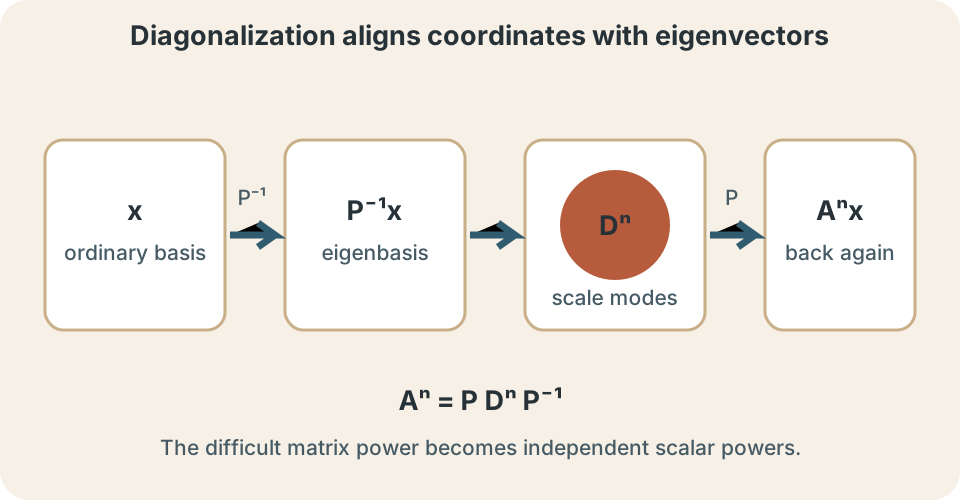
If $A$ has $n$ independent eigenvectors, place them as columns of matrix $P$. Put corresponding eigenvalues in the same order along diagonal matrix $D$. The eigenvector equations combine into $AP=PD$. Multiplying by $P^{-1}$ gives $A=PDP^{-1}$. Invertibility of $P$ comes from independent columns.

The factorization describes a change of coordinates. Matrix $P^{-1}$ converts an ordinary-coordinate vector into eigenvector coordinates. Matrix $D$ scales each eigen-coordinate independently. Matrix $P$ converts back. The diagonal action is simple because axes align with invariant directions.

Column order matters only through matching. If eigenvectors are reordered, diagonal entries must be reordered the same way. Scaling an eigenvector column changes $P$ but not the underlying diagonalization if the inverse adjusts accordingly. There is usually no unique $P$. The transformation $A$ remains fixed.

Powers become easy in diagonal form

From $A=PDP^{-1}$, square the matrix: $A^2=PDP^{-1}PDP^{-1}=PD^2P^{-1}$. The middle product $P^{-1}P$ becomes identity. Repeating gives $A^n=PD^nP^{-1}$ for nonnegative integer $n$. Diagonal powers are computed entry by entry. This cancellation is the computational advantage of the factorization.

If $D=\operatorname{diag}(\lambda_1,\ldots,\lambda_n)$, then $D^n=\operatorname{diag}(\lambda_1^n,\ldots,\lambda_n^n)$. Each eigenmode evolves independently. Large powers emphasize eigenvalues with larger magnitude, provided the starting vector has a component in those directions. Zero components remain absent. Equal magnitudes can prevent one mode from dominating.

For the earlier matrix, decompose a starting vector into the two eigendirections. After $n$ steps, its $\lambda=3$ component gains factor $3^n$. Its $\lambda=2$ component gains factor $2^n$. The ratio makes the first direction dominate for large $n$ unless that component was initially zero. Dominance is a statement about both spectrum and initial condition.

Repeated transformations and long-term behavior

Discrete dynamics often use $\mathbf x_{k+1}=A\mathbf x_k$. Here subscript $k$ counts steps. Repeated substitution gives $\mathbf x_k=A^k\mathbf x_0$. Eigenvalues predict growth, decay, reversal, or neutral behavior by mode. Initial vector determines which modes are present.

If every eigenvalue magnitude is less than one and the matrix has suitable structure, trajectories approach zero. An eigenvalue magnitude greater than one creates an expanding mode. Eigenvalue $-1$ produces sign alternation without magnitude change along its eigendirection. Eigenvalue one preserves that component. Initial coefficients determine whether each available behavior actually appears.

These simple statements need refinement for defective matrices and nonnormal behavior. Jordan blocks can introduce polynomial factors such as $k\lambda^k$. Transient growth can occur even when eigenvalues eventually predict decay. Eigenvalues remain central but do not answer every finite-time question alone. Model context matters.

Continuous-time linear systems

For differential system $\mathbf x'(t)=A\mathbf x(t)$, an eigenpair generates a modal solution $\mathbf x(t)=e^{\lambda t}\mathbf v$. Differentiate to get $\mathbf x'(t)=\lambda e^{\lambda t}\mathbf v$. Apply $A$ to get $A\mathbf x=e^{\lambda t}A\mathbf v=\lambda e^{\lambda t}\mathbf v$. Both sides match. The eigenvalue equation makes the separation possible.

A negative real eigenvalue produces exponential decay. A positive real eigenvalue produces exponential growth. A zero eigenvalue produces a constant mode. Multiple modes combine linearly when eigenvectors form a basis. Initial conditions determine coefficients.

Units matter in applications. If $t$ is seconds, eigenvalue $\lambda$ in $e^{\lambda t}$ must have unit $\mathrm{\frac{1}{s}}$ so the exponent is dimensionless. An eigenvector carries the state variable’s relative component structure. A numerical eigenvalue without time units is incomplete when matrix $A$ represents rates. Scaling time changes the numerical eigenvalues.

Complex eigenvalues encode rotation and scaling

A real $2\times2$ matrix can have complex conjugate eigenvalues $\lambda=\alpha\pm i\beta$. Real solutions combine the conjugate modes. Factor $e^{\alpha t}$ controls growth or decay. Trigonometric factors involving $\beta t$ create oscillation or rotation. The pair acts together in the real plane.

For pure rotation by angle $\theta$, eigenvalues are $e^{\pm i\theta}$. Their magnitudes are one. There may be no real invariant direction except in special angles. Complex eigenvectors live in a complexified vector space. The real transformation still acts on real vectors.

In continuous systems, complex pair with negative real part produces spiraling decay. Positive real part produces spiraling growth. Zero real part produces neutral oscillation in an ideal model. Nonlinear terms and forcing can alter the full system. Linear eigenvalues describe local or linear behavior.

Symmetric matrices have special structure

A real symmetric matrix satisfies $A^\mathsf T=A$. Its eigenvalues are real. Eigenvectors from distinct eigenvalues are orthogonal. It admits an orthonormal eigenvector basis. This is the spectral theorem.

With orthonormal eigenvectors, matrix $P$ is orthogonal. Then $P^{-1}=P^\mathsf T$. Diagonalization becomes $A=PDP^\mathsf T$. Coordinate changes preserve lengths and angles. Computation and geometry both simplify.

Covariance matrices, quadratic forms, and many vibration models use symmetric matrices. Their eigenvectors define principal directions. Their eigenvalues quantify variation, curvature, or modal stiffness depending on context. The same algebra receives different physical interpretation. Units and model definitions decide which one.

Eigenstructure in vibration and data

In coupled vibration systems, natural modes are shapes that oscillate without changing their relative component pattern. A generalized eigenvalue problem often has form $K\mathbf v=\omega^2M\mathbf v$. Matrix $K$ represents stiffness and $M$ mass. Eigenvalue $\omega^2$ determines squared angular frequency. Eigenvector $\mathbf v$ gives the mode shape.

In principal component analysis, covariance eigenvectors identify orthogonal directions of variation. Eigenvalues quantify variance along those directions. Ordering them from largest to smallest ranks captured variation. Data centering and scaling affect the result. Statistical interpretation requires more than matrix computation.

Markov-chain transition matrices also use eigenstructure. Eigenvalue one can correspond to a stationary distribution under appropriate conventions. Other eigenvalue magnitudes influence convergence rates. Probability constraints and matrix orientation matter. Application language must be mapped carefully onto the algebra.

Numerical computation and conditioning

Hand calculation via characteristic polynomials works for small matrices. It becomes unstable and impractical for large ones. Numerical algorithms use methods such as QR iteration, power iteration, or specialized symmetric solvers. Software should exploit matrix structure. It should not form high-degree characteristic polynomials naively.

Computed eigenvalues and eigenvectors contain rounding error. Residual norms test whether $A\mathbf v\approx\lambda\mathbf v$. Nearby or repeated eigenvalues can make eigenvectors sensitive to perturbations. A subspace may be well determined even when individual basis vectors are not. Conditioning deserves attention.

Normalize eigenvectors when comparisons require a standard length. Common choice is $\|\mathbf v\|_2=1$. Sign still remains arbitrary because $\mathbf v$ and $-\mathbf v$ represent the same eigendirection. Complex vectors also have arbitrary phase. Software outputs may differ while being equally valid.

Common misconceptions and repairs

One misconception allows the zero vector as an eigenvector. Zero satisfies every scale equation but supplies no direction. Exclude it explicitly. The eigenspace contains zero, but the eigenvector set removes it. Terminology matters.

Another misconception assumes eigenvalues equal diagonal entries for every matrix. That shortcut holds for triangular matrices. General matrices require the characteristic equation or an equivalent method. Trace and determinant provide checks, not a full list by inspection. Verify proposed values.

A third misconception assumes repeated eigenvalues automatically provide repeated independent eigenvectors. Geometric multiplicity can be smaller than algebraic multiplicity. Compute each null space. Count independent basis vectors. Diagonalization requires a complete basis, not merely enough roots counted with repetition.

A reliable solution routine

Confirm that $A$ is square. Form $A-\lambda I$ carefully by subtracting $\lambda$ only from diagonal entries. Compute and factor $\det(A-\lambda I)$. Solve for eigenvalues with multiplicities. Check their sum and product when trace and determinant make that convenient.

For each eigenvalue, row-reduce $A-\lambda I$. Parameterize its null space. State a basis for the eigenspace. Exclude the zero vector when naming eigenvectors. Verify at least one basis vector in $A\mathbf v=\lambda\mathbf v$.

Count independent eigenvectors before claiming diagonalization. Match columns of $P$ with entries of $D$. Use the factorization only after verifying $AP=PD$. Interpret sign, magnitude, units, and initial-mode coefficients in context. Report numerical residuals for approximate results.

Practice and connection forward

For diagonal matrix $\operatorname{diag}(4,-1,0)$, eigenvalues are $4,-1,0$. Coordinate axes are eigenvector directions. The first direction expands by four. The second reverses without changing magnitude. The third collapses to zero.

For $A=\begin{bmatrix}2&1\\1&2\end{bmatrix}$, multiply by $\begin{bmatrix}1\\1\end{bmatrix}$. The result is $\begin{bmatrix}3\\3\end{bmatrix}=3\begin{bmatrix}1\\1\end{bmatrix}$. Therefore the vector is an eigenvector with eigenvalue three. Direct multiplication is the definitive check. The vector’s direction remains on the line $y=x$.

An eigenvalue $\frac{1}{2}$ scales its mode by $\left(\frac{1}{2}\right)^{10}=\frac{1}{1024}$ after ten applications. Without looking back, derive the characteristic equation and distinguish both multiplicities. Phase-plane lessons will turn real and complex eigenvalues into trajectory types. Differential-equation lessons will use eigenmodes to construct coupled solutions. Vibration models will interpret eigenvectors as natural mode shapes.