Matrices and Linear Transformations

A matrix is more than a rectangular arrangement of numbers. It is a coordinate representation of a transformation that accepts vectors, combines their components, and produces new vectors. This input-output viewpoint explains why columns matter, why matrix multiplication uses row-column products, why multiplication order matters, and why some matrices have inverses. It also connects systems of equations to geometry and computation. Once a matrix is understood as an action, its rules become consequences rather than isolated recipes.

Learning objectives and the transformation viewpoint

By the end of this lesson, you will determine whether a transformation is linear and construct its standard matrix from basis-vector images. You will interpret matrix-vector multiplication as a linear combination of columns and matrix-matrix multiplication as composition. You will connect row reduction to systems, rank, column space, null space, and invertibility. You will explain geometric transformations through their effects on a grid, area, orientation, and special directions. You will also preserve units and verify computations through multiple representations.

We write $T:\mathbb R^n\to\mathbb R^m$ to say that transformation $T$ accepts vectors with $n$ real components and returns vectors with $m$ real components. The arrow indicates the direction from the domain to the codomain. If a matrix $A$ represents $T$, then $A$ has $m$ rows and $n$ columns. This shape is written $m\times n$, read as $m$ by $n$. The number of columns must match the input dimension, while the number of rows matches the output dimension. Matrix dimensions therefore encode the transformation’s allowed inputs and outputs.

The central formula is $T(\mathbf x)=A\mathbf x$. The bold symbol $\mathbf x$ denotes an input vector, $A$ stores the transformation in chosen coordinates, and the product produces the output. Changing the coordinate basis can change the matrix even when the underlying transformation remains the same. A matrix should therefore be interpreted together with its domain, codomain, and bases. Those contextual choices give every row and column a specific meaning.

Define linearity through preserved combinations

A transformation $T$ is linear when it preserves vector addition and scalar multiplication. These requirements are $T(\mathbf u+\mathbf v)=T(\mathbf u)+T(\mathbf v)$ and $T(c\mathbf v)=cT(\mathbf v)$ for all allowed vectors and scalars. The first property is additivity, and the second is homogeneity. Together they imply $T(c_1\mathbf v_1+\cdots+c_k\mathbf v_k)=c_1T(\mathbf v_1)+\cdots+c_kT(\mathbf v_k)$. Linear transformations therefore preserve every linear combination.

Setting the scalar $c$ equal to zero shows that every linear transformation must satisfy $T(\mathbf0)=\mathbf0$. This condition is necessary but not sufficient for linearity. A function can send zero to zero while failing to preserve addition or scaling elsewhere. It is nevertheless a fast way to reject many candidates. Any transformation that moves the origin cannot be linear in the ordinary vector-space sense.

For example, $T(x,y)=(2x-y,3y)$ is linear because each output component is a homogeneous linear combination of the inputs. In contrast, $S(x,y)=(2x-y+1,3y)$ is not linear because $S(0,0)=(1,0)$ rather than $(0,0)$. The added constant creates a translation. Such a map is affine and remains geometrically useful, but it requires a different representation or augmented coordinates. Naming the distinction prevents misuse of linear theorems.

Let basis vectors determine the entire map

The standard basis of $\mathbb R^n$ consists of vectors $\mathbf e_1,\ldots,\mathbf e_n$, each having one component equal to one and all others equal to zero. Every input has the unique expansion $\mathbf x=x_1\mathbf e_1+\cdots+x_n\mathbf e_n$. By linearity, $T(\mathbf x)=x_1T(\mathbf e_1)+\cdots+x_nT(\mathbf e_n)$. Thus knowing the images of the basis vectors determines the image of every vector. A finite list of outputs specifies the entire linear map.

The standard matrix places $T(\mathbf e_j)$ in column $j$. If $A=[T(\mathbf e_1)\ T(\mathbf e_2)\ \cdots\ T(\mathbf e_n)]$, then multiplying by $\mathbf x$ forms the required column combination. The first input coordinate weights the first column, the second coordinate weights the second column, and so forth. Columns are therefore transformed basis directions rather than arbitrary vertical lists. This interpretation should accompany every matrix-vector product.

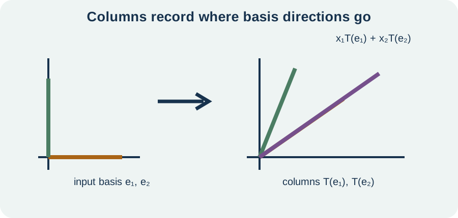
Suppose $T(\mathbf e_1)=(2,1)$ and $T(\mathbf e_2)=(-1,3)$. Then $A=\begin{bmatrix}2&-1\\1&3\end{bmatrix}$. For $\mathbf x=(4,2)$, the output is $4(2,1)+2(-1,3)=(8,4)+(-2,6)=(6,10)$. Direct matrix multiplication produces the same result. The column calculation explains why the algorithm works.

Compute a matrix-vector product with meaning

For an $m\times n$ matrix $A$ and a vector $\mathbf x\in\mathbb R^n$, the product $A\mathbf x$ lies in $\mathbb R^m$. The inner dimensions match because the number of columns of $A$ equals the number of components of $\mathbf x$. The output can be computed as a linear combination of columns. It can also be computed one row at a time using dot products. Both views produce the same vector and illuminate different structure.

Let $A=\begin{bmatrix}1&2\\0&1\end{bmatrix}$ and $\mathbf x=(3,-1)^T$. Column reasoning gives $3(1,0)+(-1)(2,1)=(1,-1)$. Row reasoning gives first component $1(3)+2(-1)=1$ and second component $0(3)+1(-1)=-1$. The superscript $T$ indicates that the ordered pair is displayed as a column. The matching answers verify the calculation.

Matrix-vector multiplication is not entrywise multiplication. An entrywise product would produce a matrix of the same shape and would not represent the stated transformation. Each output component must combine an entire row with the input vector. Equivalently, every input component must scale its corresponding column. A dimension check and a column reconstruction prevent the entrywise mistake.

Build familiar geometric transformations

A counterclockwise rotation by angle $\theta$ sends $\mathbf e_1=(1,0)$ to $(\cos\theta,\sin\theta)$. It sends $\mathbf e_2=(0,1)$ to $(-\sin\theta,\cos\theta)$. Placing these images as columns gives $R_\theta=\begin{bmatrix}\cos\theta&-\sin\theta\\\sin\theta&\cos\theta\end{bmatrix}$. The trigonometric functions encode the coordinates of unit directions after rotation. Every other vector follows by linearity.

Reflection across the $x$-axis keeps $\mathbf e_1$ fixed and sends $\mathbf e_2$ to $-\mathbf e_2$. Its matrix is $\begin{bmatrix}1&0\\0&-1\end{bmatrix}$. A horizontal scaling by factor $a$ and vertical scaling by factor $b$ has matrix $\begin{bmatrix}a&0\\0&b\end{bmatrix}$. A shear can keep one basis vector fixed while sliding the other. These matrices are easiest to construct from basis images rather than memorized templates.

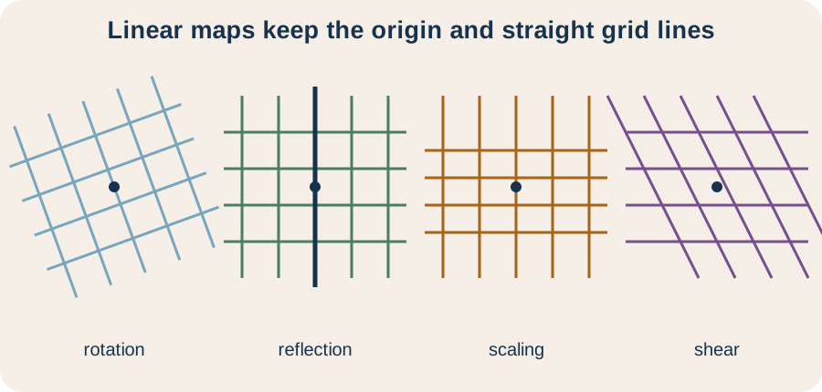
A true linear transformation maps lines through the origin to lines or to the zero vector. It preserves parallelism and ratios along a line, although it need not preserve lengths or angles. Grid lines remain straight and evenly spaced after transformation. Curved images or a moved origin signal a nonlinear or affine action. Visual invariants provide a strong check on a proposed matrix.

Interpret matrix multiplication as composition

Suppose $S(\mathbf x)=B\mathbf x$ maps an input into an intermediate space and $T(\mathbf y)=A\mathbf y$ maps that intermediate vector onward. Applying $S$ first and then $T$ gives $(T\circ S)(\mathbf x)=A(B\mathbf x)=(AB)\mathbf x$. The symbol $\circ$ denotes composition. The product $AB$ therefore represents the combined transformation. The rightmost matrix acts first.

Dimensions encode whether composition is possible. If $B$ is $p\times n$ and $A$ is $m\times p$, then $AB$ is $m\times n$. The shared dimension $p$ describes the intermediate vector space. If the inner dimensions do not match, the output of the first map cannot serve as input to the second. Matrix multiplication is undefined in that order.

Order generally matters because transformations interact differently when reversed. Scaling and then translating is not even a purely linear comparison unless augmented coordinates are used, while rotating and then reflecting can differ from reflecting and then rotating. In matrix language, $AB$ usually does not equal $BA$. Equality in special cases must be demonstrated rather than assumed. Composition explains noncommutativity as a consequence of process order.

Derive row-column matrix multiplication

To find column $j$ of $AB$, apply $A$ to column $j$ of $B$. The $j$th column of $B$ is where the composed transformation sends basis vector $\mathbf e_j$ after the first stage. Applying $A$ completes the second stage. Therefore each product column is a linear combination of columns of $A$ using entries from the corresponding column of $B$. This column rule follows directly from composition.

Entrywise, $(AB)_{ij}=\sum_{k=1}^{p}a_{ik}b_{kj}$. The subscript $ij$ identifies row $i$ and column $j$ of the product. The index $k$ runs across the shared intermediate dimension. Each term multiplies one entry from row $i$ of $A$ by the matching entry from column $j$ of $B$. Sigma adds those contributions to produce one output entry.

The algorithm should be paired with a size prediction. Multiplying an $m\times p$ matrix by a $p\times n$ matrix produces an $m\times n$ matrix. The outer dimensions give the product shape, and the matching inner dimensions permit it. After computing, test one product column by applying the two transformations sequentially to a basis vector. That check reconnects arithmetic to meaning.

Connect matrices to systems of equations

The equation $A\mathbf x=\mathbf b$ represents a linear system. Each row of $A$ supplies coefficients for one scalar equation, the vector $\mathbf x$ contains unknowns, and $\mathbf b$ contains the right-hand sides. From the column viewpoint, the same equation asks whether $\mathbf b$ is a linear combination of the columns of $A$. System consistency is therefore equivalent to membership in the column space. One notation unifies equations and span.

Elementary row operations swap equations, multiply an equation by a nonzero scalar, or add a multiple of one equation to another. These operations preserve the solution set because each can be reversed. Row echelon form exposes pivot positions and free variables. A contradictory row such as $[0\ 0\ \cdots\ 0\mid c]$ with $c\ne0$ proves inconsistency. A free variable produces infinitely many solutions when the system is consistent.

Row operations change the displayed columns and therefore do not preserve the column space as a literal set in the same coordinate space. They do preserve relationships needed to solve the system and preserve the row space. To find a basis for the original column space, identify pivot column positions in the reduced form and select those columns from the original matrix. This distinction prevents a subtle but common error. Reduction is an equation-solving tool, not a geometric deformation of the original output space.

Understand rank, nullity, and reachable outputs

The rank of a matrix is the dimension of its column space, which also equals the number of pivots. Rank counts the independent output directions the transformation can produce. A map from $\mathbb R^n$ to $\mathbb R^m$ can have rank at most the smaller of $m$ and $n$. Repeated or dependent columns do not increase rank. Rank measures effective dimensional reach rather than matrix size alone.

The null space is the set of inputs satisfying $A\mathbf x=\mathbf0$. A nonzero vector in the null space is a direction collapsed to zero by the transformation. The nullity is the dimension of that set. For a matrix with $n$ columns, the rank-nullity theorem states $\operatorname{rank}(A)+\operatorname{nullity}(A)=n$. Every input direction contributes either to independent output reach or to freedom lost in the kernel, with the theorem quantifying the balance.

If a transformation from $\mathbb R^3$ has rank two, its outputs lie in a plane-like two-dimensional subspace. At least one independent input direction is lost because nullity is one. Different inputs separated by a null-space vector produce the same output. This explains why recovering the original input may be impossible. Rank and nullity translate pivot counts into information loss.

Determine when an inverse exists

For a square matrix $A$, an inverse $A^{-1}$ satisfies $A^{-1}A=AA^{-1}=I$. The identity matrix $I$ leaves every vector unchanged. If $A\mathbf x=\mathbf b$, multiplying by the inverse gives $\mathbf x=A^{-1}\mathbf b$. This resembles division by a number, but matrix inverses exist only under specific conditions. Matrix order must also be preserved.

The invertible matrix theorem connects several equivalent statements for an $n\times n$ matrix. The matrix is invertible exactly when it has a pivot in every row and column, rank $n$, trivial null space, independent columns, and columns spanning $\mathbb R^n$. It is also equivalent to having a unique solution for every right-hand side. These are different views of the same no-information-loss condition. Proving any one establishes all the others.

Computationally, elimination is usually preferable to forming an inverse solely to solve one system. To calculate an inverse explicitly, row reduce the augmented matrix $[A\mid I]$ until the left side becomes $I$. If successful, the right side becomes $A^{-1}$. If the left side cannot reach $I$, the matrix is singular and has no inverse. Always verify a computed inverse by multiplication.

Use determinant as a geometric scale factor

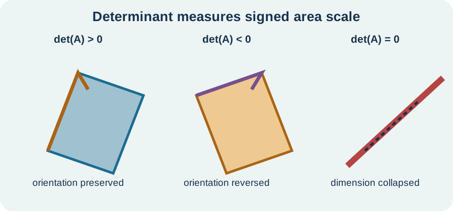
For a $2\times2$ matrix $A=\begin{bmatrix}a&b\\c&d\end{bmatrix}$, the determinant is $\det(A)=ad-bc$. This scalar measures the signed area scale factor of the transformation. If a region has area $K$, its image has area $|\det(A)|K$. A negative determinant reverses orientation, while a positive determinant preserves orientation. A zero determinant collapses area into a line or point.

The matrix is invertible exactly when its determinant is nonzero. A zero determinant means the transformed basis vectors are dependent and fail to span the plane. The associated parallelogram has zero area because its sides are parallel or one is zero. This geometric collapse explains the loss of an input direction. The determinant criterion is therefore more than an algebraic shortcut.

Determinants multiply under composition: $\det(AB)=\det(A)\det(B)$. The total area scale of two successive transformations is the product of their individual scales. If either determinant is zero, the composition cannot recover lost dimension. For higher-dimensional square matrices, determinant measures signed volume scaling. The same conceptual role persists even when the formula becomes more involved.

Track units through matrix models

Matrix entries may carry units when a transformation connects different physical quantities. If an input vector contains times in seconds and an output contains distances in meters, relevant matrix entries must have units of meters per second. Each row-column product must yield the unit of its output component. Terms added within one output component must share units. Dimensional consistency can reveal a transposed matrix or misplaced coefficient.

Consider a linear sensor model $\mathbf y=A\mathbf x$ where input concentrations are measured in milligrams per liter and outputs are voltages. Matrix sensitivities then have units $\frac{\mathrm V}{\mathrm{mg/L}}$. Multiplying sensitivity by concentration gives volts, and sums across species remain volts. Writing the horizontal fraction makes the conversion structure explicit. A dimensionless matrix is appropriate only when input and output units or normalized coordinates justify it.

Changes of basis are often dimensionless because they redescribe the same vector in different coordinate directions. Even then, basis vectors themselves may carry physical units. Mixing coordinates relative to different bases without the appropriate conversion matrix is invalid. State what each row and column represents before interpreting entries. Units and labels turn an abstract array into a reproducible model.

Verify a transformation in four complementary ways

Begin with dimensions and definitions. Confirm the domain, codomain, matrix shape, input format, and coordinate bases. If linearity is claimed, test preservation of combinations or construct the rule from homogeneous linear expressions. Check that the origin maps to the origin. A shape error often exposes a conceptual mismatch before calculation.

Next, use basis and column checks. Apply the matrix to each standard basis vector and verify that the outputs equal its columns. For a general input, recompute the product as a column combination. If matrices are composed, test the product on one basis vector by performing both transformations separately. These checks are small but structurally decisive.

Finally, compare algebra with geometry and invariants. Examine rank, determinant, null space, lengths, or angles according to what the transformation is supposed to preserve. Substitute a proposed solution into $A\mathbf x=\mathbf b$. Verify an inverse by multiplying in both orders when feasible. Several independent checks provide stronger evidence than repeating the same arithmetic.

Diagnose common misconceptions

Matrix multiplication is not entrywise multiplication and generally does not commute. Its row-column rule comes from composition and linear combinations. Reversing factors reverses the order of transformations and may make the dimensions invalid. Predict the product’s domain and codomain before multiplying. Meaning controls the algorithm.

A translation is not linear unless the translation vector is zero. It may preserve lines and shapes, but it does not preserve the zero vector or arbitrary linear combinations. Computer graphics often represents translations with homogeneous coordinates and larger matrices. That technique embeds affine transformations into a higher-dimensional linear framework. It does not change the original definition of linearity.

An inverse should never be used before existence is established. A square shape alone is insufficient, and a nearly singular matrix may create numerical sensitivity even when a theoretical inverse exists. Check pivots, determinant, or equivalent conditions. For solving systems, prefer stable elimination or factorization methods. Symbolic legality and numerical wisdom are related but distinct questions.

Practice construction, composition, and interpretation

Find the standard matrix for reflection across the $x$-axis. Begin by applying the transformation to $\mathbf e_1$ and $\mathbf e_2$. Place those images in the correct columns. Apply the matrix to a general vector $(x,y)$ and interpret the result. Verify that applying the reflection twice gives the identity transformation.

Let $A=\begin{bmatrix}1&2\\0&1\end{bmatrix}$ and $B=\begin{bmatrix}0&-1\\1&0\end{bmatrix}$. Compute $AB$ and $BA$, then describe why the products differ. Apply both products to $\mathbf e_1$ to check their first columns. Identify the geometric role of $B$ and the shear-like role of $A$. State which transformation acts first in each product.

Analyze $C=\begin{bmatrix}1&2\\2&4\end{bmatrix}$. Find its rank, determinant, and a nonzero vector in its null space. Describe the column space geometrically. Decide whether $C\mathbf x=\mathbf b$ has a unique solution for every $\mathbf b\in\mathbb R^2$. Connect every conclusion to the dependence between columns.

Solutions and reasoning

Reflection keeps $\mathbf e_1=(1,0)$ and sends $\mathbf e_2=(0,1)$ to $(0,-1)$. Its matrix is $R=\begin{bmatrix}1&0\\0&-1\end{bmatrix}$. Multiplication gives $R(x,y)^T=(x,-y)^T$, which preserves the horizontal coordinate and reverses the vertical coordinate. Computing $R^2=I$ shows that two reflections restore every input. This also proves $R^{-1}=R$.

The products are $AB=\begin{bmatrix}2&-1\\1&0\end{bmatrix}$ and $BA=\begin{bmatrix}0&-1\\1&2\end{bmatrix}$. Matrix $B$ rotates vectors counterclockwise by ninety degrees. In $AB$, $B$ acts first and $A$ then shears the rotated result. In $BA$, the shear acts first and the rotation acts second. The differing first columns equal the two distinct images of $\mathbf e_1$.

Matrix $C$ has dependent columns because the second is twice the first, so its rank is one. Its determinant is $1(4)-2(2)=0$. The vector $(-2,1)$ lies in the null space because $C(-2,1)^T=\mathbf0$. The column space is the line spanned by $(1,2)$. The transformation is not invertible and cannot produce a unique solution for every target.

Connect transformations to eigenvectors and dynamics

An eigenvector is a nonzero direction that a linear transformation preserves, although it may stretch, shrink, or reverse that direction. The equation $A\mathbf v=\lambda\mathbf v$ says that applying $A$ has the same effect as scalar multiplication by eigenvalue $\lambda$. This converts a vector action into a simpler scalar action along a special direction. Eigenvectors help reveal repeated transformation behavior. They are the natural next step after understanding matrices as maps.

Repeated applications produce $A^2,A^3$, and higher powers. These powers model multistep population changes, network transitions, iterative algorithms, and discretized dynamical systems. Composition order and stability then become central. Eigenvalues often determine whether repeated states grow, decay, oscillate, or remain steady. The geometry developed here provides the language for interpreting those outcomes.

The durable workflow is to begin with the action rather than the array. Identify input and output spaces, determine what happens to basis vectors, assemble columns, and interpret multiplication as combination or composition. Then use rank, nullity, determinant, and inverse to diagnose information preservation. A matrix becomes intelligible when every computational rule is tied to the transformation it represents. Meaning should lead the calculation and return to interpret its result.