Potential Energy

Potential energy is energy associated with the configuration of interacting parts of a system. Raising an object changes the separation between the object and Earth, while compressing a spring changes the relative positions of material within the spring. The energy belongs to the chosen system and its configuration rather than to a lone object in isolation. Conservative interactions allow work to be represented through changes in a scalar potential-energy function. This lesson develops that representation, its reference choices, and its limits.

Define the system before assigning potential energy

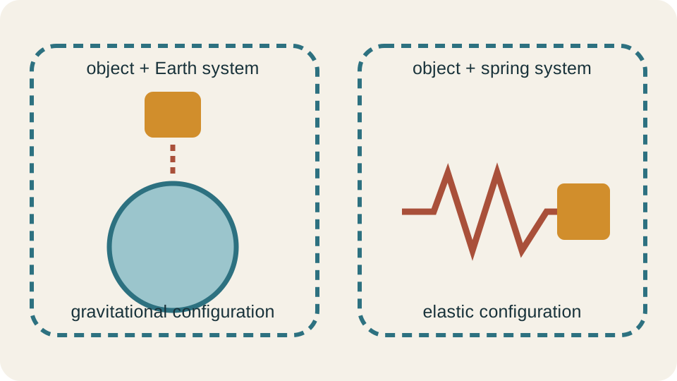
A system is the collection of objects or matter included in an energy account. Gravitational potential energy belongs to an object-Earth system because gravity is an interaction between both bodies. Elastic potential energy belongs to a system containing the deformable spring and the objects needed to define its configuration. Naming only “the object” can hide the interaction responsible for storage. System boundaries make ownership of energy explicit.

Potential energy is associated with configuration. Configuration means the relative positions, separations, orientations, or internal arrangements of interacting parts. Moving an entire isolated system without changing its internal configuration need not change its potential energy. Changing separation within the system can. The relevant coordinate depends on the interaction being modeled.

The word “stored” is useful but can mislead if imagined as a substance placed inside one object. Energy is a scalar accounting quantity. A spring system has more elastic potential energy when deformed relative to a reference configuration. An object-Earth system has a different gravitational potential energy when separation changes. The accounting follows interactions and state, not a visible material fluid.

Connect conservative work with potential change

For a conservative interaction, potential-energy change is defined by $\Delta U=-W_{\mathrm{cons}}$. The symbol $U$ denotes potential energy. The change $\Delta U=U_f-U_i$ is final minus initial potential energy. The work $W_{\mathrm{cons}}$ is work done by the conservative force during the same change. The minus sign connects energy released by the potential account with positive work by the force.

If gravity does positive work while an object falls, gravitational potential energy decreases. If an external agent raises the object slowly, gravity does negative work and potential energy increases. A compressed spring pushing an object outward does positive work while elastic potential energy decreases. Motion against a conservative force raises the corresponding potential. Motion with the force lowers it.

This relation concerns work by the conservative interaction, not automatically work by every force. Friction, drag, and an applied push may also transfer or transform energy. A complete system account includes those processes separately. Potential energy is a convenient representation for selected conservative interactions. It does not erase other energy pathways.

Recognize conservative interactions

A force is conservative when its work between two configurations depends only on the endpoints. The path taken between those endpoints does not change the conservative work. Equivalently, work around a closed path is zero. Gravity in many mechanical models and an ideal spring force are conservative. Kinetic friction is not conservative because its work depends on path length.

Path independence makes a single-valued potential-energy function possible. If two routes between the same configurations produced different conservative work, one endpoint value of $U$ could not represent both. A potential function compresses path information into state information. This is why energy methods can replace detailed force integration for conservative interactions. The endpoint difference contains the needed work result.

Real interactions may be modeled conservatively only under stated conditions. Air resistance can make mechanical energy decrease along a path. A real spring may exhibit hysteresis, so loading and unloading follow different force curves. Frictional heating can shift energy into internal accounts. Model validity must be checked against the physical process.

Derive force from a potential function

In one dimension, a conservative force is related to potential energy by $F_x=-\dfrac{dU}{dx}$. The derivative $dU/dx$ is the slope of the potential-energy graph. Its units are joules per meter. Since one joule per meter equals one newton, the derivative has force units. The negative sign makes force point toward decreasing potential energy.

If $U$ rises as $x$ increases, then $dU/dx$ is positive and $F_x$ is negative. The force points back toward smaller $x$. If $U$ falls as $x$ increases, the slope is negative and force is positive. A horizontal potential segment has zero force. Graph slope therefore encodes both force magnitude and direction.

In three dimensions, the relation becomes $\mathbf F=-\boldsymbol\nabla U$. The gradient $\boldsymbol\nabla U$ points in the direction of steepest potential increase. The force points opposite that gradient. Component relations are $F_x=-\partial U/\partial x$, $F_y=-\partial U/\partial y$, and $F_z=-\partial U/\partial z$. The one-dimensional formula is the simplest case of this spatial rule.

Choose a reference level

Potential energy is defined up to an additive constant. If $U(x)$ is a valid potential, then $U'(x)=U(x)+C$ produces the same force because the derivative of constant $C$ is zero. The prime here labels an alternative function rather than a derivative. Physical motion depends on differences in $U$. The zero level can therefore be chosen for convenience.

For near-Earth gravity, a tabletop, floor, or launch point may be assigned $U_g=0$. A different zero changes every listed potential value by the same constant. It does not change $\Delta U_g$. Kinetic-energy predictions and forces remain unchanged. Reference choice is bookkeeping, not a physical alteration.

A stated reference prevents ambiguous numbers. Saying an object has $50.0\,\mathrm{J}$ of gravitational potential energy is incomplete without the zero level and system. Saying it has $50.0\,\mathrm{J}$ relative to the floor is clearer. For astronomical gravity, zero is often chosen at infinite separation. Different problems may use different convenient conventions.

Model near-Earth gravitational potential energy

Near Earth’s surface over modest height changes, gravitational force magnitude is approximately constant. The potential-energy change is $\Delta U_g=mg\Delta y$. Mass $m$ is measured in kilograms, gravitational-field magnitude $g$ in meters per square second, and vertical displacement $\Delta y$ in meters. The product has units $\mathrm{kg\,m^2/s^2}$, which equal joules. Positive upward displacement increases potential energy.

With a chosen zero at $y=0$, the function can be written $U_g(y)=mgy$. This form is a local approximation to the more general gravitational potential. Its derivative is $dU_g/dy=mg$. Therefore the vertical gravitational force is $F_y=-mg$ when positive $y$ points upward. The derivative relation reproduces the familiar downward weight.

Suppose a $3.00\,\mathrm{kg}$ object rises by $2.00\,\mathrm{m}$ where $g=9.81\,\mathrm{\dfrac{m}{s^2}}$. Then $\Delta U_g=(3.00\,\mathrm{kg})(9.81\,\mathrm{\dfrac{m}{s^2}})(2.00\,\mathrm{m})=58.9\,\mathrm{J}$. The positive result means the object-Earth configuration gained potential energy. Gravity did $-58.9\,\mathrm{J}$ of work during the rise. An external process must account for the corresponding transfer when motion begins and ends at the same speed.

Understand the limits of m g y

The expression $mgy$ assumes nearly constant gravitational field strength and a vertical coordinate measured over a region small compared with Earth’s radius. It is excellent for rooms, hills, and many laboratory trajectories. It becomes inaccurate for large altitude changes or planetary-scale motion. Then gravitational strength changes appreciably with separation. A more general potential is required.

For two pointlike or spherically symmetric masses, gravitational potential energy is $U(r)=-\dfrac{GMm}{r}$ when zero is chosen at infinite separation. The symbol $G$ is the universal gravitational constant. The coordinate $r$ is center-to-center separation. The negative sign indicates that a bound finite-separation configuration lies below the zero at infinity. Increasing $r$ raises $U$ toward zero.

The local $mg\Delta y$ relation can be recovered as an approximation over a small radial interval. Near Earth’s surface, the slope magnitude of $-GMm/r$ is approximately $mg$. The two formulas are not competing truths. One is a broad inverse-distance model, and the other is its local constant-field approximation. Scale determines which representation is appropriate.

Model elastic potential energy

An ideal spring obeys Hooke’s law $F_x=-kx$, where $x$ is displacement from equilibrium. The spring constant $k$ has units newtons per meter. The negative sign indicates a restoring force opposite the displacement. The model assumes a range where force is proportional to deformation. Real springs depart from it when stretched or compressed too far.

The potential-energy function is $U_s(x)=\dfrac{1}{2}kx^2$ when zero is chosen at equilibrium. Differentiating gives $dU_s/dx=kx$, so $F_x=-dU_s/dx=-kx$. The square makes energy nonnegative for either compression or extension under this reference. Equal-magnitude deformations store equal elastic potential energy. Direction appears in force, not in the scalar energy magnitude.

A spring with $k=250\,\mathrm{\dfrac{N}{m}}$ compressed by $0.0800\,\mathrm{m}$ stores $U_s=\dfrac{1}{2}(250\,\mathrm{\dfrac{N}{m}})(0.0800\,\mathrm{m})^2=0.800\,\mathrm{J}$. Units reduce as $(\mathrm{N/m})(\mathrm{m^2})=\mathrm{N\,m}=\mathrm{J}$. The deformation should be measured from the spring’s equilibrium length. Using total spring length instead would misidentify the coordinate. The answer is unchanged for an equal $0.0800\,\mathrm{m}$ extension because the deformation is squared.

Interpret the one-half factor

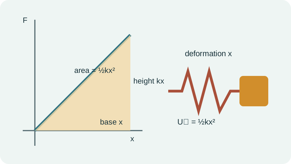
Spring force is not constant during compression. It grows in magnitude from zero at equilibrium to $kx$ at final displacement. Work against the spring equals the area under the applied-force versus displacement graph in a slow process. That graph is a triangle with base $x$ and height $kx$. Its area is $\dfrac{1}{2}x(kx)=\dfrac{1}{2}kx^2$.

Using $W=Fd$ with the final force $kx$ would overestimate work by a factor of two. The average force during linear loading is $\dfrac{0+kx}{2}=\dfrac{kx}{2}$. Multiplying this average by displacement gives the correct result. The horizontal fraction bar groups the changing-force average. Geometry and integration agree.

More generally, work is $W=\int F_x\,dx$. The integral sign represents accumulated contributions from continuously changing force. For the spring, integrating $kx$ from zero to $x$ gives $\dfrac{1}{2}kx^2$. The one-half factor records the linear increase in force. It is not an arbitrary constant to memorize.

Use potential-energy diagrams

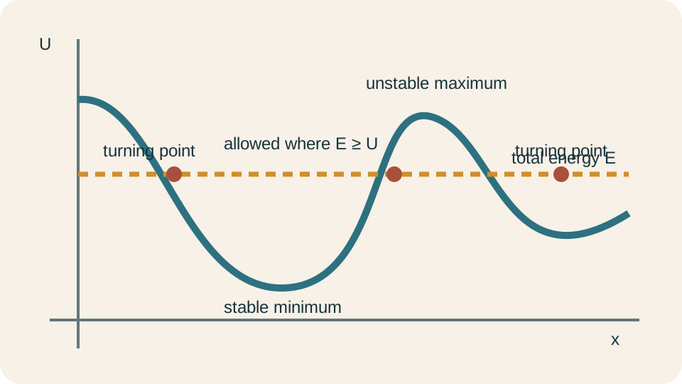
A potential-energy diagram plots $U(x)$ vertically against configuration coordinate $x$ horizontally. The graph’s height is energy, while its slope determines force through $F_x=-dU/dx$. The graph is not necessarily a picture of a physical hill. A horizontal coordinate could represent separation, deformation, or another generalized configuration. Reading axes prevents a metaphor from replacing the model.

Equilibrium occurs where force is zero, so $dU/dx=0$. A local minimum represents stable equilibrium because a small displacement raises potential and produces a restoring force. A local maximum represents unstable equilibrium because a small displacement lowers potential and drives the system farther away. A flat region can indicate neutral equilibrium or weak restoring behavior. Curvature near equilibrium influences oscillation stiffness.

If total mechanical energy $E$ is drawn as a horizontal line, classically allowed positions satisfy $E\geq U(x)$ because kinetic energy $K=E-U$ cannot be negative. Turning points occur where $E=U$ and kinetic energy momentarily reaches zero. The object can reverse there. Higher gaps $E-U$ correspond to greater kinetic energy and therefore greater speed for fixed mass. Regions where $U>E$ are inaccessible under the stated classical mechanical-energy account.

Combine kinetic and potential accounts

Kinetic energy of translational motion is $K=\dfrac{1}{2}mv^2$. Rotational kinetic energy can also be present as $K_{\mathrm{rot}}=\dfrac{1}{2}I\omega^2$. The symbol $I$ is rotational inertia, and $\omega$ is angular speed. Introductory problems often omit rotational motion because objects are modeled as particles or because rotation is negligible. It must be included when wheels, pulleys, rolling bodies, or rotating machinery store a meaningful share of energy.

Mechanical energy is commonly defined as $E_{\mathrm{mech}}=K+U$ for selected kinetic and potential accounts. If only internal conservative forces exchange energy and no external transfer occurs, mechanical energy remains constant. A decrease in $U$ appears as an increase in $K$. An increase in $U$ requires energy from kinetic or another transfer. The balance describes conversion within the chosen system.

Friction can shift mechanical energy into internal energy. External work can transfer energy across the system boundary. Chemical reactions, electrical processes, heating, and radiation may contribute additional accounts. Writing only $K_i+U_i=K_f+U_f$ is justified only when omitted transfers and accounts are negligible. System and process analysis must precede the simplified equation.

Distinguish potential energy from force

Potential energy is a scalar measured in joules. Force is a vector measured in newtons. A large potential value does not necessarily imply a large force. Force depends on the spatial slope of potential, not its absolute height. A high flat plateau can have zero force.

Potential energy can be negative under a chosen reference without being physically impossible. Only differences affect classical motion. Gravitational potential with zero at infinity is negative for bound finite separations. Adding a constant can shift all values while leaving force unchanged. Negative potential is not negative total energy automatically.

Force direction is recovered through the negative gradient. Potential itself has no direction. Saying potential energy “points downward” is therefore incorrect. The gravitational force points downward in a near-Earth coordinate system, while gravitational potential increases upward. Scalars and vectors play complementary but distinct roles.

Include chemical and internal configurations

Chemical potential energy is associated with electromagnetic interactions and molecular arrangement. Reaction products and reactants can have different internal energy because their configurations and bonding differ. Introductory diagrams often use the phrase “chemical energy stored in fuel.” A more precise account assigns this energy to the material system and its microscopic configuration. Reaction pathways transfer energy among internal, mechanical, thermal, and environmental accounts. The system boundary determines whether that transfer appears as an internal conversion or energy crossing the boundary.

No universal elementary formula like $mgy$ or $\dfrac{1}{2}kx^2$ describes all chemical energy changes. Values often come from measured reaction enthalpies, bond-energy approximations, or detailed quantum models. The configuration principle remains relevant, but the interaction is more complex. Using a mechanical formula outside its domain would be unjustified. Models must match the physical scale and process.

Internal energy includes microscopic kinetic and potential contributions. Molecular translation, rotation, vibration, intermolecular arrangement, and electronic states can contribute. Heating can change these accounts without changing macroscopic height or spring deformation. Potential energy in mechanics is one part of a broader energy framework. Clear account labels prevent “stored energy” from becoming a vague catch-all.

Track multiple potential contributions

A system can contain several conservative interactions. Its total potential may be $U=U_g+U_s+U_{mathrm{other}}$. Each term must use compatible units and a clearly chosen reference. Adding potentials is valid because energy is scalar. Forces then add through the negative derivative or gradient of the total potential.

Consider a hanging mass attached to a vertical spring. With upward coordinate $y$, gravitational potential may be $mgy$. Spring deformation depends on how $y$ relates to spring equilibrium length. The total potential can be differentiated to locate equilibrium. Choosing coordinates carefully prevents inconsistent signs.

At equilibrium, the spring’s restoring force balances weight. In a suitable coordinate, differentiating total potential reproduces $kx=mg$ for the equilibrium extension magnitude. Expanding the total potential near that minimum describes oscillations about equilibrium. Energy and force methods reach the same physical condition. The potential approach often makes stability more visible.

Diagnose common potential-energy errors

One mistake is assigning gravitational potential energy to an isolated object without including Earth conceptually. The interaction requires both. Another is treating the chosen zero as physically privileged. Shifting every potential value by a constant does not change predictions. Only differences enter the work relation.

Another mistake is using $mgh$ regardless of scale. The constant-field approximation fails for very large changes in altitude. A related mistake is inserting horizontal displacement into $mg\Delta y$. Only vertical separation changes the near-Earth potential. Path length does not replace vertical coordinate change.

A spring error is using total length instead of deformation from equilibrium. Another is omitting the square or one-half factor. Unit checks expose some of these mistakes because $kx$ has force units while $kx^2$ has energy units. A diagram and derivative check expose the rest. Formula selection must follow the configuration definition.

Practice a complete energy analysis

Suppose a $0.500\,\mathrm{kg}$ block begins $1.20\,\mathrm{m}$ above a chosen zero level and compresses a spring with $k=300\,\mathrm{\dfrac{N}{m}}$ by $0.100\,\mathrm{m}$. Its initial gravitational potential relative to the zero is $U_g=(0.500\,\mathrm{kg})(9.81\,\mathrm{\dfrac{m}{s^2}})(1.20\,\mathrm{m})=5.89\,\mathrm{J}$. The compressed spring stores $U_s=\dfrac{1}{2}(300\,\mathrm{\dfrac{N}{m}})(0.100\,\mathrm{m})^2=1.50\,\mathrm{J}$. These values belong to their defined system configurations. Both results are expressed in joules, so they can enter one energy balance.

If the block begins and ends at rest and the spring is the only receiver of mechanical energy, $1.50\,\mathrm{J}$ cannot account for the full $5.89\,\mathrm{J}$ gravitational decrease. The missing $4.39\,\mathrm{J}$ must appear in another account or indicate inconsistent geometry. It could become kinetic energy, internal energy through friction, sound, or work across the boundary. Energy accounting reveals missing physics. It does not permit energy to disappear.

A complete routine names the system, initial and final states, reference levels, and transfers. It writes each energy term with units. It includes translational and rotational kinetic energy when relevant. It checks whether simplified conservation assumptions match the process. The numerical equation comes after the physical account is constructed.

Consolidate potential-energy reasoning

Potential energy represents configuration within a chosen interacting system. Conservative work equals the negative change in potential. Force points down the potential gradient. Reference levels shift absolute values without changing differences or motion. Units and derivatives connect the scalar potential to measurable forces.

Near-Earth gravity uses $\Delta U_g=mg\Delta y$ under a constant-field approximation. Ideal springs use $U_s=\dfrac{1}{2}kx^2$ within their linear range. More general gravitational, chemical, and internal configurations require other models. Potential diagrams reveal force direction, equilibrium, stability, allowed regions, and turning points. Each representation answers a specific question.

The strongest energy solution begins with system definition and configuration. It chooses an appropriate potential, states a reference, tracks all relevant accounts, and checks units. It includes rotation when an extended object moves rotationally rather than silently treating every body as a particle. Potential energy is powerful because it replaces conservative path details with state differences. Its power depends on careful boundaries, assumptions, and interpretation.