Hooke’s Law

Stretch a spring slightly and it pulls back. Compress it slightly and it pushes outward. In a useful range, the restoring force is proportional to displacement from equilibrium and points in the opposite direction. Hooke’s law expresses that pattern with one constant called stiffness. The model is powerful because many stable systems behave approximately linearly near equilibrium.

Hooke’s law is not a universal rule for every deformation. Real springs can curve away from proportional behavior, dissipate energy, fatigue, or deform permanently. A rubber band does not usually have one constant stiffness over a large stretch. Experimental force–displacement data must establish the useful range. The model’s limitations are part of its meaning.

This lesson develops the law from equilibrium, signs, and graphs. It then derives elastic potential energy and combines springs in series and parallel. Worked examples will carry force, displacement, and stiffness units. An experimental section will distinguish uncertainty from genuine nonlinearity. The final connection will show why a linear restoring force produces simple harmonic motion.

Learning objectives and an opening prediction

After this lesson, you should define equilibrium and signed displacement. You should apply $F_s=-kx$ without treating the negative sign as a negative magnitude. You should determine stiffness from a force–displacement graph and assess linearity. You should derive and calculate elastic potential energy. You should also find equivalent stiffness for ideal series and parallel arrangements.

Imagine identical springs stretched by $0.020\,\mathrm m$ and $0.060\,\mathrm m$ within their linear ranges. Predict the force-magnitude ratio. Since force magnitude is $kx$, tripling displacement triples force. The more stretched spring also stores nine times the energy because energy depends on $x^2$. Force and energy therefore scale differently with displacement.

Now imagine pulling a spring beyond the point where it returns to its original length. Hooke’s law has not become algebraically wrong; its physical assumptions have failed. A permanent offset indicates plastic deformation. A curved loading graph indicates changing effective stiffness. Model validation requires observing the material after unloading as well as during loading.

Equilibrium is the reference point

Equilibrium is a configuration where the net force is zero. Define signed displacement $x$ from that configuration. The choice $x=0$ belongs at equilibrium, not automatically at the spring’s natural length. Other forces can shift equilibrium. A vertical hanging mass is a common example.

For an isolated horizontal ideal spring, natural length and equilibrium can coincide. For a vertical spring holding mass $m$, static equilibrium satisfies $k x_0=mg$. Here $x_0$ is the downward extension from natural length. If subsequent motion is described by displacement $y$ from the hanging equilibrium, gravity cancels the constant spring contribution. The net restoring force becomes $F_{\mathrm{net}}=-ky$.

Choosing the equilibrium-centered coordinate simplifies both signs and equations. Positive direction may be right, left, up, or down. Once chosen, it must remain consistent. A negative coordinate means position lies opposite the positive direction. It is not a negative distance or an impossible deformation.

Hooke’s law contains magnitude and direction

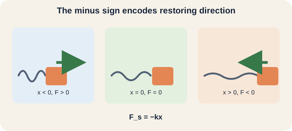
Hooke’s law in one dimension is $F_s=-kx$. The symbol $F_s$ is the spring-force component in newtons. The constant $k$ is positive and measured in newtons per meter, $\mathrm{\frac{N}{m}}$. Displacement $x$ is measured in meters from equilibrium. The negative sign states that force and displacement have opposite signs.

If $x=+0.030\,\mathrm m$ and $k=200\,\mathrm{\frac{N}{m}}$, then $F_s=-(200\,\mathrm{\frac{N}{m}})(+0.030\,\mathrm m)=-6.0\,\mathrm N$. The negative result means force points in the negative direction. If $x=-0.030\,\mathrm m$, then $F_s=+6.0\,\mathrm N$. The force magnitudes match because the displacement magnitudes match. In both cases, force points toward equilibrium.

Force magnitude can be written $|F_s|=k|x|$. This form is useful when a problem asks only how strong the force is. It discards direction and should not be substituted into a signed Newton’s-law equation. Vector notation in several dimensions may be written $\mathbf F_s=-k\mathbf x$ only for an isotropic ideal restoring relation. More general systems require stiffness matrices or direction-specific constants.

A graph tests proportionality

Plot spring force $F_s$ vertically against displacement $x$ horizontally. Hooke’s law predicts a straight line through the origin with slope $-k$. The slope units are $\mathrm{\frac{N}{m}}$. A larger slope magnitude means a stiffer spring. The negative slope encodes restoring direction.

Some experiments instead plot applied force magnitude against extension magnitude. Under slow equilibrium loading, applied force balances the spring force, so the graph has positive slope $+k$. This is not a contradiction because the plotted force and sign convention changed. Both graphs yield the same positive stiffness magnitude. Axis labels must name “spring force” or “applied force.” A graph without that distinction is ambiguous.

Use a best-fit line across the supported linear range. Do not calculate stiffness from one noisy ratio unless only one measurement exists. Residuals should scatter without systematic curvature if a straight-line model is appropriate. A nonzero intercept may indicate a zeroing error, preload, friction, or an incorrect reference point. Evidence decides whether to adjust the apparatus or the model.

Measuring stiffness in a static experiment

Hang known masses from a vertical spring and allow each to settle. At static equilibrium, upward spring-force magnitude equals downward weight, so $kx=mg$. The applied load is therefore $F=mg$. Measure extension from the same reference for every trial. Avoid oscillating readings by waiting for motion to decay.

Suppose a $0.200\,\mathrm{kg}$ mass produces extension $0.0650\,\mathrm m$. Its weight magnitude is $F=(0.200\,\mathrm{kg})(9.81\,\mathrm{\frac{m}{s^2}})=1.96\,\mathrm N$. A one-point estimate is $k=\frac{1.96\,\mathrm N}{0.0650\,\mathrm m}=30.2\,\mathrm{\frac{N}{m}}$. The horizontal fraction bar keeps force above displacement. Multiple loads provide a stronger estimate.

Measurement uncertainty affects both axes. Mass uncertainty changes calculated force, while ruler resolution and parallax affect extension. Repeating load and unload cycles can reveal hysteresis. Never exceed a safe extension merely to make the graph larger. An experiment must protect both equipment and people.

Elastic potential energy comes from accumulated work

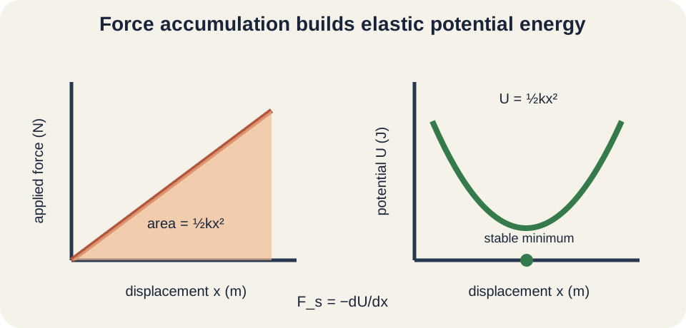
The force needed to stretch an ideal spring slowly has magnitude $F_{\mathrm{applied}}=kx$. It grows from zero rather than remaining constant. Work done by the applied force from zero to $x$ is the area under the applied-force versus displacement graph. That graph is a triangle with base $x$ and height $kx$. The stored elastic potential energy is therefore $U_s=\frac{1}{2}kx^2$ when $U_s(0)=0$.

Calculus gives the same result: $U_s(x)-U_s(0)=\int_0^x kx'\,dx'=\frac{1}{2}kx^2$. The primed $x'$ is a dummy integration variable, not a derivative. The factor one half appears because force increases linearly from zero to its final magnitude. Using $W=Fx$ with the final force would double the correct result. Variable force requires area or integration.

The spring force relates to potential energy by $F_s=-\frac{dU_s}{dx}$. Differentiating $U_s=\frac{1}{2}kx^2$ gives $\frac{dU_s}{dx}=kx$. The negative sign then recovers $F_s=-kx$. Force points downhill on the potential-energy curve. Stable equilibrium is the minimum at $x=0$.

Worked example: stiffness and stored energy

A spring extends $0.0600\,\mathrm m$ under a steady $18.0\,\mathrm N$ pull. At equilibrium the spring-force magnitude equals the applied force. Stiffness is $k=\frac{18.0\,\mathrm N}{0.0600\,\mathrm m}=300\,\mathrm{\frac{N}{m}}$. The units show force required per meter of extension. The result assumes the point lies within a linear range established by data.

At $x=0.0400\,\mathrm m$, stored energy is $U_s=\frac{1}{2}(300\,\mathrm{\frac{N}{m}})(0.0400\,\mathrm m)^2=0.240\,\mathrm J$. One meter cancels the denominator, leaving newton-meters, which equal joules. Squaring displacement is essential. Compression by the same magnitude stores the same ideal energy. Doubling this displacement would quadruple stored energy.

The force magnitude at $0.0400\,\mathrm m$ is $12.0\,\mathrm N$. Multiplying final force by displacement gives $0.480\,\mathrm J$, twice the stored energy. The correct average applied force during a slow linear stretch is $6.00\,\mathrm N$. Its product with $0.0400\,\mathrm m$ gives $0.240\,\mathrm J$. This comparison makes the triangular factor concrete.

Parallel springs share displacement

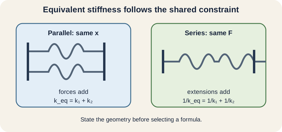
Two springs in parallel connect the same moving object to a support so each undergoes the same displacement $x$. Their restoring forces add: $F_{\mathrm{total}}=-k_1x-k_2x$. Factoring gives $F_{\mathrm{total}}=-(k_1+k_2)x$. Therefore $k_{\mathrm{eq}}=k_1+k_2$. Parallel attachment is stiffer than either spring alone.

If $k_1=100\,\mathrm{\frac{N}{m}}$ and $k_2=150\,\mathrm{\frac{N}{m}}$, then $k_{\mathrm{eq}}=250\,\mathrm{\frac{N}{m}}$. A $10.0\,\mathrm N$ load produces extension $x=\frac{10.0\,\mathrm N}{250\,\mathrm{\frac{N}{m}}}=0.0400\,\mathrm m$. The first spring carries $4.00\,\mathrm N$ and the second $6.00\,\mathrm N$. Their forces sum to the load. The stiffer spring carries the larger share at the common displacement.

Equal displacement is the structural constraint that produces addition. It should be stated before writing the formula. If geometry causes different extensions, the simple parallel expression may not apply. Levers, angled springs, and moving attachment points change effective stiffness. Draw the deformation before selecting an equation.

Series springs share force

Two ideal massless springs in series carry the same force magnitude $F$ in static equilibrium. Their individual extensions are $x_1=\frac{F}{k_1}$ and $x_2=\frac{F}{k_2}$. Total extension is $x=x_1+x_2=F\left(\frac{1}{k_1}+\frac{1}{k_2}\right)$. Since $x=\frac{F}{k_{\mathrm{eq}}}$, $\frac{1}{k_{\mathrm{eq}}}=\frac{1}{k_1}+\frac{1}{k_2}$. The equivalent stiffness is smaller than either individual stiffness.

For two springs, this can be rearranged as $k_{\mathrm{eq}}=\frac{k_1k_2}{k_1+k_2}$. With $100\,\mathrm{\frac{N}{m}}$ and $150\,\mathrm{\frac{N}{m}}$, $k_{\mathrm{eq}}=60.0\,\mathrm{\frac{N}{m}}$. A $10.0\,\mathrm N$ force creates total extension $0.1667\,\mathrm m$. The softer spring extends more. Extensions add while force remains common.

Series and parallel formulas resemble resistor combinations in opposite order. Memorizing that resemblance can help but does not explain it. Springs combine according to shared force or shared displacement. Circuit resistors combine according to shared current or shared voltage. Constraint reasoning is more transferable than pattern matching.

The elastic limit and nonlinearity

The proportional limit marks where force and displacement cease to be approximately proportional. The elastic limit marks the largest deformation from which the material returns to its original configuration. These limits need not be identical. Beyond the elastic limit, plastic deformation leaves a permanent change. Hooke’s law should not be extrapolated through that region.

Real force–displacement curves may show hysteresis. Loading and unloading follow different paths, enclosing an area. That area represents mechanical energy transferred into thermal or internal structural changes per cycle. An ideal conservative spring retraces the same line and returns stored energy. Hysteresis therefore signals behavior absent from the ideal model.

Springs can also fatigue under repeated cycling below a one-time failure load. Cracks, heating, creep, and material aging change response. Stiffness may depend on deformation rate and temperature. Engineering data sheets specify allowable loads and cycles. A classroom equation is not a safety certification.

Why linear behavior appears near equilibrium

Many smooth potential-energy functions can be approximated near a stable minimum. Expand $U(x)$ near equilibrium $x=0$: the constant term sets an arbitrary energy reference, and the first derivative vanishes at the minimum. The leading changing term is approximately quadratic, $U(x)\approx U(0)+\frac{1}{2}kx^2$. Taking the negative derivative gives $F\approx-kx$. This is why Hooke-like behavior appears beyond literal metal springs.

The approximation is local. Higher-order terms such as $x^3$ and $x^4$ become important farther from equilibrium. The acceptable range depends on required accuracy. A precision instrument may detect nonlinearity that a classroom ruler cannot. “Small displacement” means small enough for the purpose and evidence.

Molecular vibrations, structural deflections, pendulum motion at small angle, and acoustic oscillations can share this mathematical structure. Their stiffness-like constants arise from different physical interactions. The common linearization produces similar equations of motion. Each application still requires its own coordinate and valid range. Recognizing structure allows knowledge to transfer across systems without erasing their differences.

Hooke’s law leads to simple harmonic motion

Combine Newton’s second law $F_{\mathrm{net}}=ma$ with $F_s=-kx$ for an ideal horizontal mass–spring system. Then $ma=-kx$, so $a=-\frac{k}{m}x$. Acceleration is proportional to displacement and oppositely directed. That is the defining condition for simple harmonic motion. The spring law supplies the restoring dynamics.

Writing $a=\frac{d^2x}{dt^2}$ gives $\frac{d^2x}{dt^2}+\frac{k}{m}x=0$. Its sinusoidal solution has angular frequency $\omega=\sqrt{\frac{k}{m}}$. A stiffer spring oscillates faster, while a larger mass oscillates slower. The ideal period is $T=2\pi\sqrt{\frac{m}{k}}$. These results depend on linearity and negligible damping.

If the force curve becomes nonlinear, period can depend on amplitude and the motion need not be sinusoidal. If damping acts, amplitude decays and mechanical energy leaves the oscillator. If external driving acts, resonance and phase lag appear. Hooke’s law is the gateway to those richer models. Its range must be tested before the resulting predictions are trusted.

Common misconceptions and repairs

One misconception says the negative sign means spring force magnitude is negative. Magnitudes are nonnegative. The sign gives direction relative to the chosen axis. Write $|F_s|=k|x|$ when only magnitude is requested. Use $F_s=-kx$ for signed dynamics.

Another misconception applies $U_s=\frac{1}{2}kx^2$ to any deformed object. The formula assumes the linear Hooke relation and a chosen zero at equilibrium. A nonlinear elastic element requires $U(x)-U(0)=\int_0^x F_{\mathrm{applied}}(x')\,dx'$. Hysteretic systems do not have one single-valued conservative energy curve. Data determine the correct area.

A third misconception adds series spring constants. Parallel constants add because displacement is shared and forces add. Series compliances, the reciprocals of stiffness, add because force is shared and extensions add. State the constraint first. The formula then follows rather than being guessed.

Practice with guided feedback

First, find force for $k=200\,\mathrm{\frac{N}{m}}$ at $x=-0.030\,\mathrm m$. Second, find stored energy at that displacement. Third, combine $120\,\mathrm{\frac{N}{m}}$ and $180\,\mathrm{\frac{N}{m}}$ springs in parallel and then in series. Fourth, explain what a curved residual pattern means in a linear fit. Include signs and units.

Force is $F_s=-(200)(-0.030)=+6.0\,\mathrm N$, pointing positive. Energy is $U_s=\frac{1}{2}(200)(0.030)^2=0.090\,\mathrm J$. Parallel stiffness is $300\,\mathrm{\frac{N}{m}}$. Series stiffness is $\frac{(120)(180)}{120+180}=72.0\,\mathrm{\frac{N}{m}}$. Systematic residual curvature suggests the constant-stiffness model does not fully describe the measured range.

For a conceptual check, compare $x$ with $-x$. The spring-force sign reverses but its magnitude remains equal. Stored energy remains the same because $x^2=(-x)^2$. Thus the ideal potential is symmetric about equilibrium. An asymmetric measured response signals a different or more complicated system.

Retrieval and connection forward

Without looking back, explain the sign in $F_s=-kx$ and define every symbol with units. Sketch both spring-force and applied-force graphs and label their slope signs. Derive $U_s=\frac{1}{2}kx^2$ from area. Derive series and parallel equivalent stiffness from their shared constraints. Finish by naming evidence that Hooke’s law has failed.

Simple harmonic motion uses this restoring law to predict sinusoidal position, period, velocity, and energy exchange. Potential-energy lessons generalize force as the negative spatial derivative of energy. Materials science distinguishes elastic, plastic, and viscoelastic response. Engineering structures use stiffness matrices for coupled directions. The local linear idea remains the common foundation.

Keep one organizing statement: Hooke’s law is a tested local model in which restoring force is proportional and opposite to displacement from equilibrium. Its slope magnitude is stiffness. Its force–displacement area gives quadratic elastic potential energy. Shared constraints determine equivalent stiffness. Its usefulness depends on staying inside the evidenced elastic linear range.