Continuity and Bernoulli’s Equation

Water speeds through a narrow hose nozzle, pressure changes along a pipe, and a tank drains under gravity. These phenomena can be organized by conservation laws. Continuity is mass conservation written for flowing material. Bernoulli’s equation is a mechanical-energy relation under a restricted ideal model. Neither is a slogan that faster flow always means lower pressure.

Fluid problems are difficult when equations are chosen before the system is modeled. One must identify inlet and outlet sections, density, elevation, flow regime, and energy-transfer devices. A pump adds mechanical energy, a turbine removes it, and viscosity transfers organized mechanical energy into internal energy. Compressibility changes the mass-volume relationship. Each condition determines which equation is valid.

This lesson begins with a control volume and derives mass flow rate. It then derives Bernoulli’s terms as energy per volume and applies them with continuity. Worked examples will include full units and sign-consistent elevations. A real-flow extension will expose losses and machinery terms. The goal is to use conservation deliberately rather than matching visual keywords.

Learning objectives and an opening prediction

After this lesson, you should distinguish volume flow rate from mass flow rate. You should derive and apply steady-flow continuity for compressible and incompressible fluids. You should interpret every Bernoulli term as pressure or energy density. You should solve coupled area–speed–pressure–height problems. You should also identify when pumps, turbines, viscosity, unsteadiness, or compressibility require a richer model.

Imagine water flowing steadily through a pipe that narrows to one quarter of its original area. Predict the new average speed under the incompressible model. Equal volume must pass each section per second, so speed becomes four times larger. This result follows from mass conservation, not from Bernoulli’s equation. Pressure cannot yet be predicted without height and energy information.

Now imagine the same narrowing contains a pump. Continuity still constrains mass flow if no fluid accumulates or leaks. The simple Bernoulli equation across the pump does not apply because shaft work enters the fluid. Faster flow and pressure can both increase if sufficient energy is added. The two conservation statements answer different parts of the problem.

A control volume organizes flowing matter

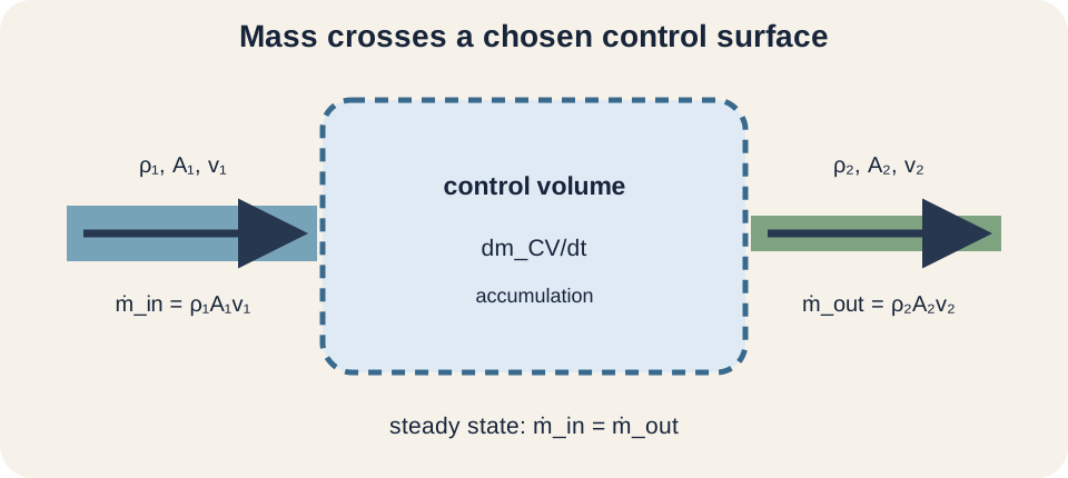
A control volume is a selected region in space through which fluid can cross. Its boundary is the control surface. Choose sections where area, average velocity, density, and pressure can be represented meaningfully. Material may enter, leave, or accumulate inside. Mass conservation compares those rates.

For one inlet and one outlet, the general mass balance is $\frac{dm_{CV}}{dt}=\dot m_{\mathrm{in}}-\dot m_{\mathrm{out}}$. The left side is the rate of mass accumulation inside the control volume. An overdot means derivative with respect to time. At steady state, properties at fixed locations do not change with time, so accumulation is zero. Then inlet and outlet mass flow rates are equal.

Steady does not mean individual fluid particles are motionless. It means measured fields such as pressure and average velocity do not change with time at each location. A river can flow steadily. Uniform means the same value across space, which is a different idea. A steady pipe flow can be spatially nonuniform because area and speed vary along it.

Volume flow rate measures volume per time

For approximately uniform velocity perpendicular to a cross-section, volume flow rate is $Q=Av$. The symbol $Q$ denotes volume per time in $\mathrm{\frac{m^3}{s}}$, $A$ is area in square meters, and $v$ is average normal speed in $\mathrm{\frac{m}{s}}$. Multiplying gives cubic meters per second. The equation follows because a fluid slab travels distance $v\Delta t$ and occupies volume $A v\Delta t$. Dividing by $\Delta t$ gives $Av$.

If velocity varies across the section, the exact relation is $Q=\int_A\mathbf v\boldsymbol\cdot d\mathbf A$. The area vector points normal to each small surface element. The dot product selects the velocity component crossing the surface. Average velocity is defined so that $Q=A v_{\mathrm{avg}}$. Elementary pipe problems usually use this cross-sectional average.

Volume flow rate is not fluid speed. A wide pipe can carry a large $Q$ at modest speed. A narrow jet can have high speed but smaller total volume rate. Liters per minute and cubic meters per second are flow-rate units, while meters per second are speed units. Dimensional analysis prevents their substitution.

Mass flow rate includes density

Mass flow rate is $\dot m=\rho Q=\rho A v$ for uniform average section properties. Density $\rho$ has units $\mathrm{\frac{kg}{m^3}}$. Multiplying by $Q$ in $\mathrm{\frac{m^3}{s}}$ gives $\mathrm{\frac{kg}{s}}$. Mass flow rate counts kilograms crossing per second. It is the quantity directly constrained by mass conservation.

For steady one-inlet, one-outlet flow, $\rho_1A_1v_1=\rho_2A_2v_2$. Subscripts one and two label sections. This relation remains useful for compressible flow when densities differ, provided representative average quantities are valid. Canceling density without justification can violate mass conservation. Gas density often changes substantially with pressure and temperature.

For an incompressible fluid, a moving material element keeps essentially constant density. Then $\rho_1=\rho_2$, and continuity reduces to $A_1v_1=A_2v_2=Q$. Liquids often approximate this behavior at moderate pressure changes. “Incompressible” is a modeling approximation, not a claim that density can never change. Its adequacy depends on required accuracy.

Worked continuity example

Water flows through area $A_1=4.00\times10^{-3}\,\mathrm{m^2}$ with average speed $v_1=2.00\,\mathrm{\frac{m}{s}}$. The pipe narrows to $A_2=1.00\times10^{-3}\,\mathrm{m^2}$. Incompressible continuity gives $A_1v_1=A_2v_2$. Solve as $v_2=\frac{A_1}{A_2}v_1$. The area ratio is dimensionless.

Substitution gives $v_2=\frac{4.00\times10^{-3}\,\mathrm{m^2}}{1.00\times10^{-3}\,\mathrm{m^2}}(2.00\,\mathrm{\frac{m}{s}})=8.00\,\mathrm{\frac{m}{s}}$. The smaller section has four times the speed. Volume flow rate is $Q=A_1v_1=(4.00\times10^{-3})(2.00)=8.00\times10^{-3}\,\mathrm{\frac{m^3}{s}}$. Cross-sectional area units multiply speed to create volume per time. The outlet product gives the same value.

With water density $1000\,\mathrm{\frac{kg}{m^3}}$, mass flow rate is $\dot m=\rho Q=(1000)(8.00\times10^{-3})=8.00\,\mathrm{\frac{kg}{s}}$. The numerical value differs from volume rate because the units and measured quantity differ. Both remain constant across the ideal steady streamtube. Density converts cubic meters per second into kilograms per second. Agreement at both sections is a conservation check.

Bernoulli’s equation is a mechanical-energy balance

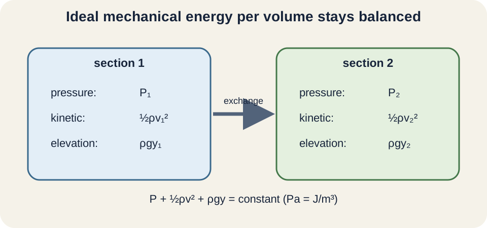
For steady, incompressible, nonviscous flow along a streamline with no pump or turbine work, Bernoulli’s equation is $P+\frac{1}{2}\rho v^2+\rho gy=\text{constant}$. The symbol $P$ is static pressure in pascals, $\rho$ is density, $v$ is speed, $g$ is gravitational acceleration, and $y$ is elevation. Each term has units of energy per volume. Their sum is evaluated for the same fluid parcel path under the model. One pascal equals one joule per cubic meter.

Between two points, write $P_1+\frac{1}{2}\rho v_1^2+\rho gy_1=P_2+\frac{1}{2}\rho v_2^2+\rho gy_2$. Writing both sides before canceling prevents omitted terms. Pressure contribution, kinetic energy density, and gravitational potential-energy density can exchange. The equation does not state that each term remains constant. It states that their sum does under the assumptions.

The pressure term represents flow work per volume associated with pushing fluid across a boundary. The dynamic term $\frac{1}{2}\rho v^2$ is kinetic energy per volume. The elevation term $\rho gy$ is gravitational potential energy per volume relative to an arbitrary zero height. Changing the height reference adds the same constant consistently and does not alter predictions. Pressure must be expressed on a consistent absolute or gauge basis.

Verify the units term by term

Pressure has units $\mathrm{Pa}=\mathrm{\frac{N}{m^2}}=\mathrm{\frac{J}{m^3}}$. For the kinetic term, $\rho v^2$ has units $\mathrm{\frac{kg}{m^3}}\mathrm{\frac{m^2}{s^2}}=\mathrm{\frac{kg}{m\,s^2}}=\mathrm{Pa}$. The factor one half is dimensionless. Thus it can be added to pressure. A unit mismatch signals an incorrect expression.

For the elevation term, $\rho gy$ has units $\mathrm{\frac{kg}{m^3}}\mathrm{\frac{m}{s^2}}\mathrm m=\mathrm{\frac{kg}{m\,s^2}}=\mathrm{Pa}$. It is also energy per volume. Calling it simply “potential energy” omits the per-volume basis. Total energy would require multiplication by a fluid volume. Consistent basis makes the equation additive.

Another common form divides by $\rho g$: $\frac{P}{\rho g}+\frac{v^2}{2g}+y=\text{constant}$. Every term then has units of meters and is called a head. Pressure head, velocity head, and elevation head are energy per unit weight. Do not mix pressure-form terms with head-form terms. Choose one complete basis.

Horizontal narrowing pipe

Return to water moving from $v_1=2.00\,\mathrm{\frac{m}{s}}$ to $v_2=8.00\,\mathrm{\frac{m}{s}}$ at equal elevations. Bernoulli gives $P_1+\frac{1}{2}\rho v_1^2=P_2+\frac{1}{2}\rho v_2^2$. Rearranging gives $P_1-P_2=\frac{1}{2}\rho(v_2^2-v_1^2)$. The faster section has lower static pressure under these stated assumptions. Continuity supplied the speeds first.

Using $\rho=1000\,\mathrm{\frac{kg}{m^3}}$, $P_1-P_2=\frac{1}{2}(1000)(8.00^2-2.00^2)=3.00\times10^4\,\mathrm{Pa}$. Squared speed units combine with density to produce pascals. The value is $30.0\,\mathrm{kPa}$. It is a pressure difference, not necessarily either absolute pressure. A boundary condition is needed to find individual pressures.

This result does not establish a universal “fast means low pressure” law. A pump can add energy, height can change, viscous loss can occur, and comparisons can involve different streamlines. Even within ideal flow, pressure and speed respond to the complete ledger. The narrowing example works because elevation and added or removed work were controlled. State those conditions with the conclusion.

Torricelli’s result for tank draining

Consider a large open tank with a small outlet a vertical distance $h$ below the free surface. Choose point one at the free surface and point two at the outlet. Both are exposed to atmospheric pressure, so their pressure terms cancel using the same reference. The tank area is much larger than outlet area, so free-surface speed is approximated as zero. Bernoulli then relates elevation loss to outlet kinetic energy.

With $y_1-y_2=h$, $\rho gh=\frac{1}{2}\rho v_2^2$. Density cancels, giving $v_2=\sqrt{2gh}$. This is Torricelli’s result. It resembles free-fall speed after dropping through height $h$ because gravitational potential energy becomes kinetic energy in the ideal model. The square root keeps speed nonnegative.

If $h=1.25\,\mathrm m$ and $g=9.81\,\mathrm{\frac{m}{s^2}}$, $v_2=\sqrt{2(9.81)(1.25)}=4.95\,\mathrm{\frac{m}{s}}$. A real outlet may discharge more slowly because of contraction and viscous losses. As the tank drains, $h$ changes, so the flow is not globally steady over long times. The outlet speed therefore decreases as the free surface falls. The result can still approximate each moment when the level changes slowly.

Static, stagnation, and dynamic pressure

Static pressure is the thermodynamic pressure a fluid exerts locally and is measured by a suitable port moving with or aligned to avoid speed conversion. Dynamic pressure is the shorthand $q=\frac{1}{2}\rho v^2$. It is not automatically an independently exerted isotropic pressure. Stagnation pressure is the pressure reached if flow slows ideally to zero at the same elevation. In horizontal incompressible ideal flow, $P_0=P+q$.

A Pitot tube faces into flow and brings fluid nearly to rest at its opening. A separate static port measures static pressure. Their difference estimates dynamic pressure. Then speed is $v=\sqrt{\frac{2(P_0-P)}{\rho}}$. Density and calibration must be known. Compressible high-speed flow needs corrected relations.

Confusing static and stagnation pressure causes erroneous claims. A moving stream can have substantial static pressure as well as kinetic energy density. Bringing it to rest converts some kinetic term into pressure under ideal conditions. The measurement apparatus changes the local flow intentionally. Probe orientation is part of the experiment.

Pumps, turbines, and real losses extend the ledger

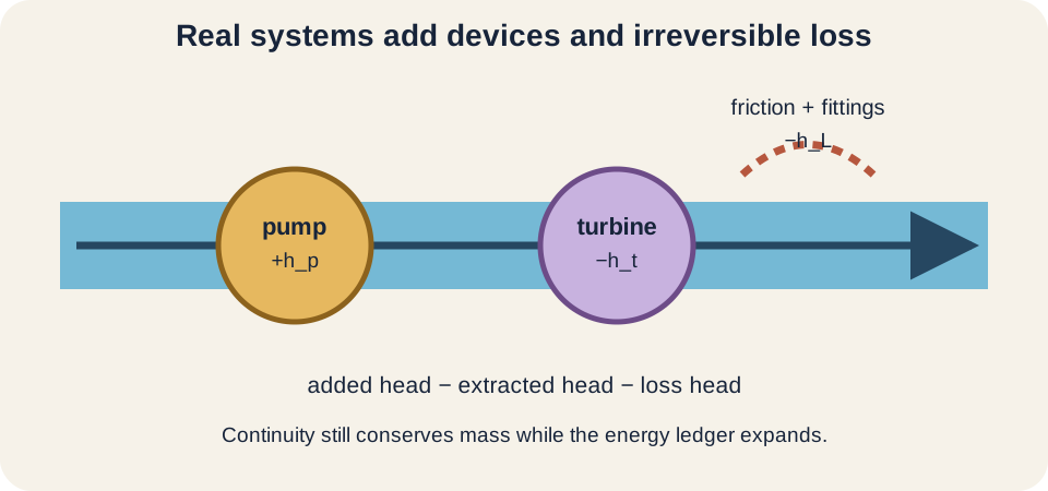
Real systems can be written in head form as $\frac{P_1}{\rho g}+\frac{v_1^2}{2g}+y_1+h_p-h_t-h_L=\frac{P_2}{\rho g}+\frac{v_2^2}{2g}+y_2$. Pump head $h_p$ adds mechanical energy per unit weight. Turbine head $h_t$ removes useful shaft energy. Loss head $h_L$ represents irreversible mechanical-energy degradation. Every term has units meters.

Viscosity creates shear and transfers organized flow energy into internal energy. In a constant-diameter horizontal pipe without a pump, speed may remain approximately constant while static pressure falls along the flow. Simple Bernoulli without a loss term would incorrectly predict equal pressure. The pressure drop drives the viscous flow. Longer pipes, smaller diameters, roughness, and higher speed often increase loss.

A pump can raise pressure while speed also increases. This directly refutes the unqualified faster-flow-lower-pressure slogan. A turbine can reduce pressure or speed while delivering shaft power. System devices must be placed inside the energy boundary. Their power relates to mass flow and head through $P\approx\eta\rho gQh$ with efficiency definitions specified.

Streamlines and rotational flow

The elementary Bernoulli constant is guaranteed along a streamline under the stated assumptions. A streamline is tangent to the instantaneous velocity field. In steady flow, streamlines coincide with particle paths. Different streamlines can have different Bernoulli constants in rotational flow. Comparing arbitrary points across them may be invalid.

If the flow is irrotational, the Bernoulli constant can be common across streamlines under appropriate conditions. Introductory problems often silently assume this stronger setting or choose points along one streamtube. A diagram should show the connection. When uncertain, restrict the application to a named streamline. Mathematical permission must accompany algebra.

Turbulence introduces rapidly fluctuating velocity and pressure. Time-averaged equations can still be used, but extra terms represent turbulent transport and losses. A single streamline may not provide a stable description. Engineering models use empirical coefficients and computational methods. The ideal equation remains a reference case rather than a complete turbulent theory.

Compressibility and high-speed flow

In gas flow, density can vary with pressure and temperature. Mass continuity $\rho Av=\dot m$ remains foundational, but $Av$ need not stay constant. The incompressible Bernoulli form also becomes inaccurate when density changes appreciably. An equation of state and compressible energy relations are then needed. Mach number helps assess compressibility importance.

For air at modest speeds, density changes may be small enough for an incompressible approximation. A common engineering guideline considers compressibility increasingly important above Mach numbers around $0.3$, though accuracy needs and conditions matter. Near sonic speed, choking and shock waves can occur. Area changes then produce behavior unlike simple liquid-nozzle intuition. The full conservation laws remain valid while simplified forms change.

Temperature can change because flow work and kinetic energy interact with internal energy. The simple Bernoulli equation tracks only mechanical forms for an incompressible idealization. Compressible-flow energy includes enthalpy explicitly. A gas nozzle can cool while accelerating. Thermodynamics supplies the broader ledger.

Viscosity and laminar pipe flow

Viscosity measures resistance to deformation rate within a fluid. In laminar pipe flow, adjacent layers slide with an orderly velocity profile. No-slip at a stationary wall makes velocity zero there, while speed is largest near the center. Average speed is therefore lower than centerline speed. Using a center speed as $v$ in $Q=Av$ overestimates flow.

For fully developed laminar flow in a circular pipe, the Hagen–Poiseuille relation connects volume flow with pressure drop, viscosity, length, and radius. Its strong radius dependence shows why narrow tubes greatly resist flow. Bernoulli alone cannot predict that pressure loss. Viscosity introduces irreversibility. A real problem may require both continuity and a viscous relation.

Reynolds number compares inertial and viscous effects. Low values tend to support laminar flow, while high values can support turbulence depending on geometry and disturbances. It is dimensionless. Flow regime determines which correlations and approximations apply. One should not assume “smooth-looking pipe” means inviscid fluid.

Common misconceptions and repairs

One misconception says narrowing creates mass. In steady incompressible flow, the same volume and mass rates cross every section, so speed adjusts inversely with area. More fluid particles do not appear in the throat. Their spatial spacing remains tied to nearly constant density. Continuity provides the correction.

Another misconception says pressure is always lower wherever speed is higher. Bernoulli relates a complete set of terms under specific assumptions. Height, pumps, losses, and comparison paths can reverse or modify the pattern. State what is held constant. Use the ledger rather than a one-line slogan.

A third misconception calls $\frac{1}{2}\rho v^2$ the fluid’s total pressure in every context. It is kinetic energy per volume and is often named dynamic pressure. Stagnation pressure includes static plus dynamic terms only in the appropriate ideal same-height case. Measurement location and probe type matter. Labels should track operational meaning.

Practice with guided feedback

First, water enters a pipe of area $6.00\times10^{-3}\,\mathrm{m^2}$ at $3.00\,\mathrm{\frac{m}{s}}$ and exits through half that area; find exit speed and $Q$. Second, find the ideal outlet speed from a tank with $h=0.800\,\mathrm m$. Third, explain why adding inertial speed alone cannot determine pressure. Fourth, name the correction needed across a pump. State the assumptions supporting every selected equation.

Continuity gives exit speed $6.00\,\mathrm{\frac{m}{s}}$ and $Q=(6.00\times10^{-3})(3.00)=1.80\times10^{-2}\,\mathrm{\frac{m^3}{s}}$. Torricelli gives $v=\sqrt{2(9.81)(0.800)}=3.96\,\mathrm{\frac{m}{s}}$. Pressure also depends on elevation, energy transfers, losses, and boundary conditions. A pump-head or shaft-work term must be added. Each result follows from an explicit model choice.

For a unit check, show that $\rho v^2$ reduces to pascals. For a direction check, verify that the smaller incompressible area has greater speed. For an energy check, verify that a lower outlet can acquire kinetic energy from elevation. For a validity check, identify whether viscosity or time dependence is negligible. These four checks catch most elementary errors.

Retrieval and connection forward

Without looking back, derive $Q=Av$ from a moving fluid slab and then derive $\dot m=\rho Av$. State compressible and incompressible continuity forms. Write Bernoulli’s equation and explain every term with units. Solve a narrowing-pipe story without invoking a universal pressure slogan. Finish by adding pump, turbine, and loss terms conceptually.

Thermodynamics expands the energy balance to enthalpy, heat transfer, shaft work, and irreversibility. Fluid dynamics develops momentum balances, boundary layers, drag, and turbulence. Circuit theory will show an analogy between pressure difference and electrical potential difference, though the analogy has limits. Biological flow applies viscous pressure loss in vessels. Engineering design combines conservation with empirical loss data.

Keep one organizing statement: continuity conserves mass, while Bernoulli conserves ideal mechanical energy along an allowed path. Area and speed couple through volume flow only when density is constant. Pressure, kinetic energy density, and elevation exchange within the Bernoulli ledger. Pumps, turbines, viscosity, turbulence, compressibility, and unsteadiness require additional terms or different equations. Conservation survives even when the simple formula does not.