Density and Pressure

Density describes how mass is distributed through volume. Pressure describes how normal force is distributed across area. These quantities answer different questions, but together they explain much of fluid statics. Density connects material amount to occupied space. Pressure connects microscopic molecular interaction to macroscopic force.

A stationary fluid supports its own weight through pressure variation. Deeper locations generally have greater pressure because more fluid lies above them. Pressure at a point acts in every direction in an ideal fluid at rest. Container shape affects forces on boundaries but does not replace depth as the central hydrostatic variable. These ideas lead directly to buoyancy, hydraulic machines, and atmospheric pressure.

This lesson develops the definitions, units, and assumptions behind density and pressure. It derives the hydrostatic equation from a force balance rather than quoting it. It distinguishes absolute, atmospheric, and gauge pressure. Worked examples include conversions and uncertainty-aware reporting. The final workflow emphasizes diagrams, system boundaries, and dimensional checks.

Learning objectives and opening comparisons

After this lesson, you should calculate average density from mass and volume. You should calculate pressure from perpendicular force and area. You should derive and apply pressure variation with depth. You should distinguish gauge from absolute pressure. You should explain Pascal’s principle without claiming that a hydraulic device creates energy.

Compare one kilogram of iron with one kilogram of foam. Their masses are equal, but the foam occupies much more volume. Iron therefore has greater average density. Density does not mean “how heavy” an object is by itself. It compares mass with occupied volume.

Now place the same book first flat and then on its narrow edge. Its weight remains nearly unchanged. The smaller contact area produces greater average pressure on the surface. Force and pressure are not synonyms. Pressure asks how concentrated the normal force is.

Density is mass per volume

Average mass density is $\rho=\frac{m}{V}$. The Greek letter $\rho$, pronounced “rho,” represents density, $m$ is mass, and $V$ is volume. SI density unit is $\mathrm{\frac{kg}{m^3}}$. Laboratory chemistry often uses $\mathrm{\frac{g}{cm^3}}$ or $\mathrm{\frac{g}{mL}}$. Every density value must include a material state and appropriate conditions when those matter.

Consider a uniform block with mass $m=2.40\,\mathrm{kg}$ and volume $V=3.00\times10^{-4}\,\mathrm{m^3}$. Divide mass by volume according to the definition. Keep the scientific-notation exponent in the denominator visible. The quotient should be larger than one because the volume is a small fraction of a cubic metre. Three significant figures are supported by both inputs. The calculation appears below.

$$\rho =\frac{2.40\,\mathrm{kg}} {3.00\times10^{-4}\,\mathrm{m^3}} =8.00\times10^3\,\mathrm{\frac{kg}{m^3}}.$$

Kilograms remain in the numerator and cubic metres in the denominator. The result has three significant figures. Its order of magnitude is typical of a dense solid. Reversing the fraction would produce the wrong dimension. The unit confirms which quantity was calculated.

Average density can hide internal variation. Local density is defined conceptually by examining mass in increasingly small volumes around a point. A fluid can have density that varies with position, temperature, or pressure. Liquids are often approximated as incompressible over modest pressure ranges. Gases usually require more attention to changing density.

Convert density units by cubing length factors

One gram per cubic centimetre is not one kilogram per cubic metre. Use $1\,\mathrm g=10^{-3}\,\mathrm{kg}$ and $1\,\mathrm{cm}=10^{-2}\,\mathrm m$. Cubing the length relation gives $1\,\mathrm{cm^3}=10^{-6}\,\mathrm{m^3}$. Therefore $1\,\mathrm{\frac{g}{cm^3}}=10^3\,\mathrm{\frac{kg}{m^3}}$. The large factor arises because volume scales with the cube of length.

Now convert $7.85\,\mathrm{\frac{g}{cm^3}}$ to SI. Replace grams with kilograms through an exact defined factor. Replace cubic centimetres with cubic metres through a cubed factor. Orient both factors so starting units cancel. Preserve the three measured significant figures. The factor-label calculation is shown below.

$$7.85\,\mathrm{\frac{g}{cm^3}} \left(\frac{10^{-3}\,\mathrm{kg}}{1\,\mathrm g}\right) \left(\frac{1\,\mathrm{cm}}{10^{-2}\,\mathrm m}\right)^3 =7.85\times10^3\,\mathrm{\frac{kg}{m^3}}.$$

Grams and cubic centimetres cancel. The remaining unit is the desired SI form. The numerical magnitude increases by $10^3$. This does not mean the material became denser. Only the unit representation changed.

A common error is applying the centimetre-to-metre factor only once. That would convert length rather than volume. Write the unit exponent before choosing conversion factors. If an area appears, square the factor. If a volume appears, cube it.

Pressure is normal force per area

Average pressure is $P=\frac{F_\perp}{A}$. The symbol $P$ is pressure, $F_\perp$ is force perpendicular to a surface, and $A$ is area. Tangential force contributes shear stress rather than ordinary pressure. Pressure is a scalar field in a fluid, though the force it produces on a surface has direction. Surface orientation determines the force direction.

The SI unit of pressure is the pascal. One pascal is $1\,\mathrm{Pa}=1\,\mathrm{\frac{N}{m^2}}$. Using $\mathrm N=\mathrm{\frac{kg\,m}{s^2}}$ gives $\mathrm{Pa}=\mathrm{\frac{kg}{m\,s^2}}$. Atmospheric pressures are often reported in kilopascals because one pascal is small. Standard atmosphere is approximately $101.325\,\mathrm{kPa}$.

If a perpendicular force of $600\,\mathrm N$ acts uniformly over $0.0200\,\mathrm{m^2}$, average pressure is $\frac{600\,\mathrm N}{0.0200\,\mathrm{m^2}}=3.00\times10^4\,\mathrm{Pa}$. If the area halves while force remains fixed, pressure doubles. The total force has not increased. It has become more concentrated. A nonuniform contact would require a local pressure distribution rather than this single average.

Pressure at a point acts in all directions

In an ideal fluid at rest, pressure at a point is isotropic. This means its value does not depend on the orientation of a tiny test surface through that point. If pressure differed by direction, an infinitesimal fluid element would experience unbalanced torque or motion. Static equilibrium forbids that persistent imbalance. Molecular collisions supply normal forces on any boundary orientation.

Pressure itself has no arrow direction. The force on a surface element is normal to that surface. A vertical wall feels a horizontal pressure force, while a horizontal floor feels a vertical pressure force. The same scalar pressure can therefore generate differently directed forces. Geometry converts a field value into boundary force.

For a small flat area under nearly uniform pressure, force magnitude is $F=PA$. For varying pressure, use $dF=P\,dA$ and integrate across the surface. The differential area $dA$ identifies a small patch. Direction can vary on curved surfaces. Large-wall problems require both pressure variation and geometry.

Derive hydrostatic pressure variation

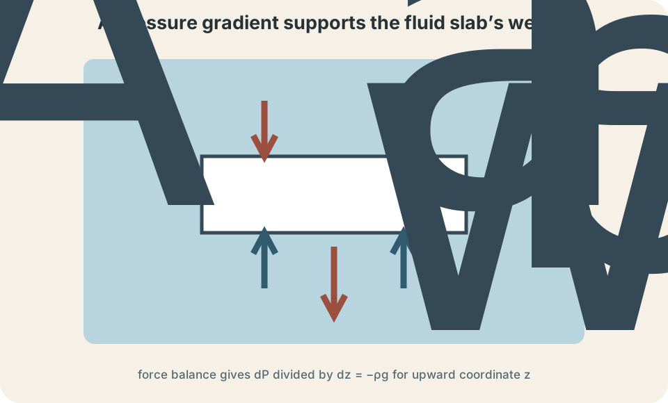
Consider a stationary fluid slab with horizontal area $A$ and thickness $dz$. Let upward coordinate be $z$. Pressure on the bottom pushes upward with force $P(z)A$. Pressure on the top pushes downward with force $P(z+dz)A$. The slab’s weight is approximately $\rho gA\,dz$ downward.

Vertical force balance gives $P(z)A-P(z+dz)A-\rho gA\,dz=0$. Divide by $A\,dz$ and take the thin-slab limit. The result is $\frac{dP}{dz}=-\rho g$. Pressure decreases as upward coordinate increases. Equivalently, pressure increases with downward depth.

If density and gravitational acceleration are constant, integrate between two levels. For depth $h$ below a free surface, $P=P_{\mathrm{surface}}+\rho gh$. The symbol $h$ is positive downward depth. The term $\rho gh$ is the pressure increase produced by the overlying fluid. The formula assumes a static incompressible fluid and approximately constant $g$.

Depth, not container shape, sets hydrostatic pressure

At equal depth in the same connected stationary fluid, pressure is equal under the standard assumptions. A narrow tube and a wide tank can have the same pressure at their bottoms if their free surfaces are at the same height. The total force on each bottom can differ because areas differ. Pressure equality does not imply force equality. This distinction resolves the hydrostatic paradox.

Container walls exert forces on the fluid. In a flaring container, wall forces can have vertical components. These forces help balance the difference between fluid weight and bottom force. Looking only at the bottom can make the force seem too large or too small. The whole container–fluid force balance restores consistency.

Pressure does not depend directly on the total amount of fluid. A very narrow tall column can create large bottom pressure with modest fluid volume. A broad shallow pool can contain enormous volume but have lower bottom pressure if depth is smaller. Depth determines the local hydrostatic increase. Area determines how that pressure becomes a total force.

Worked depth example with units

Find absolute pressure $5.00\,\mathrm m$ below a freshwater surface open to the atmosphere. Use $\rho=1.00\times10^3\,\mathrm{\frac{kg}{m^3}}$, $g=9.81\,\mathrm{\frac{m}{s^2}}$, and $P_{\mathrm{atm}}=1.013\times10^5\,\mathrm{Pa}$. The pressure increase is $\Delta P=\rho gh$. Every numerical value includes units. First calculate the water contribution separately from the atmospheric reference.

Multiply density, gravitational acceleration, and depth. The depth is positive because it is measured downward from the surface. The product should have pressure units. Keep the atmospheric term out of this intermediate step. This separation distinguishes gauge from absolute pressure. The calculation follows.

$$\Delta P =\left(1.00\times10^3\,\mathrm{\frac{kg}{m^3}}\right) \left(9.81\,\mathrm{\frac{m}{s^2}}\right) (5.00\,\mathrm m) =4.91\times10^4\,\mathrm{Pa}.$$

The unit reduces to $\mathrm{\frac{kg}{m\,s^2}}$, which is pascals. The result is gauge pressure relative to the surface atmosphere. Greater depth would increase this contribution linearly under the model. Zero depth would make it zero. These limiting cases support the sign and form.

Absolute pressure is $P_{\mathrm{abs}}=P_{\mathrm{atm}}+\Delta P=1.50\times10^5\,\mathrm{Pa}$ after rounding. Water density was treated as constant. Surface waves and atmospheric variation were neglected. At much greater depth, compressibility and varying $g$ can require refinement. Assumptions set the accuracy of the model.

Absolute, atmospheric, and gauge pressure

Absolute pressure is measured relative to an ideal vacuum. It cannot be negative in ordinary thermodynamic interpretation. Atmospheric pressure is the local pressure exerted by the atmosphere. Gauge pressure is measured relative to local atmospheric pressure. The relationship is $P_{\mathrm{gauge}}=P_{\mathrm{abs}}-P_{\mathrm{atm}}$.

A tire gauge commonly reports gauge pressure. If it reads $220\,\mathrm{kPa}$ where atmospheric pressure is $101\,\mathrm{kPa}$, absolute tire pressure is $321\,\mathrm{kPa}$. Reporting “tire pressure is $220\,\mathrm{kPa}$” is ambiguous without naming the reference. Instruments often embed that reference in their design. Scientific reporting should make it explicit.

Negative gauge pressure means absolute pressure is below atmospheric pressure. It does not mean negative absolute pressure. Suction language often refers to this pressure difference. Atmospheric pressure then pushes fluid or an object toward the lower-pressure region. A vacuum cleaner does not pull by a mysterious inward force; pressure imbalance produces net force.

Manometers compare pressures

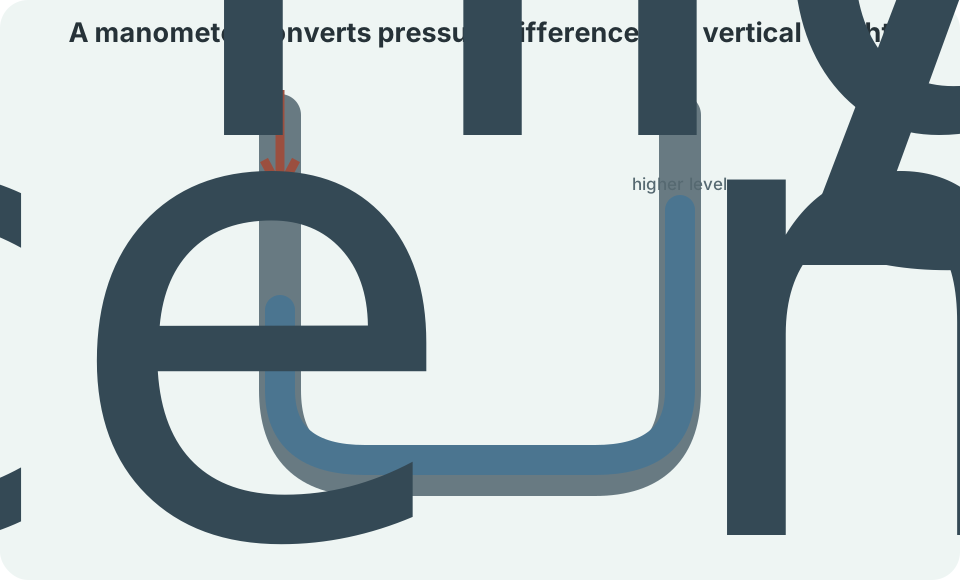
A U-tube manometer contains a fluid whose height difference responds to pressure difference. If both arms contain the same manometer fluid and other density effects are negligible, $\Delta P=\rho g\Delta h$. The symbol $\Delta h$ is the vertical level difference. The higher-pressure side depresses the fluid there. Sign follows the chosen pressure order.

Suppose mercury with density $13.6\times10^3\,\mathrm{\frac{kg}{m^3}}$ has height difference $0.120\,\mathrm m$. The pressure difference magnitude is $(13.6\times10^3)(9.81)(0.120)\,\mathrm{Pa}$. This equals $1.60\times10^4\,\mathrm{Pa}$. Density, gravity, and vertical height must use compatible units. The higher-pressure side is identified by the depressed mercury level.

When different fluids occupy the arms, trace pressure step by step. Moving downward through a fluid increases pressure by $\rho g\Delta h$. Moving upward decreases it. Pressure is continuous across a stationary interface apart from surface-tension effects neglected in the elementary model. A labeled path prevents sign errors.

Pascal’s principle and hydraulic systems

Pascal’s principle states that a pressure change applied to a confined fluid is transmitted throughout the fluid under static conditions. In an ideal hydraulic system, input and output gauge pressures are equal at equal elevation. Thus $\frac{F_1}{A_1}=\frac{F_2}{A_2}$. A larger output area produces a larger output force. This is force multiplication.

If $A_2=20A_1$, then ideally $F_2=20F_1$. The device does not multiply energy. Volume conservation gives $A_1\Delta x_1=A_2\Delta x_2$ for incompressible fluid. The larger output force moves through a proportionally smaller distance. Ideally $F_1\Delta x_1=F_2\Delta x_2$.

Real hydraulic systems have friction, fluid compressibility, leakage, and structural deformation. These reduce efficiency and alter response. Elevation differences add hydrostatic pressure terms. Dynamic operation adds flow effects. Pascal’s principle begins the model rather than eliminating engineering details.

Atmospheric pressure comes from a fluid column

Earth’s atmosphere has weight and therefore produces pressure. A simple constant-density model would give $\Delta P=\rho gh$, but air density changes strongly with altitude. Hydrostatic balance still gives $\frac{dP}{dz}=-\rho g$. An equation of state relates density to pressure and temperature. Integrating then produces an altitude profile.

At sea level, standard atmospheric pressure is $101325\,\mathrm{Pa}$. This equals $101.325\,\mathrm{kPa}$ by definition of kilo. It is also approximately one atmosphere. Actual weather and altitude cause variation. A barometer measures atmospheric pressure through a supported fluid column or another calibrated mechanism.

Drinking through a straw illustrates pressure difference. Lowering pressure in the mouth and straw lets atmospheric pressure on the liquid surface push liquid upward. The mouth does not pull liquid from a distance. The maximum height is limited by available atmospheric pressure and liquid density. Vapor pressure and flow losses can reduce practical performance.

Pressure and density in compressible fluids

Liquids often undergo small density changes under ordinary pressure variations. The incompressible approximation treats $\rho$ as constant. Gases change volume more readily, so density can vary substantially with pressure and temperature. Applying $P=P_0+\rho gh$ with one constant gas density across a tall atmosphere is inaccurate. The differential equation must be integrated with variable $\rho$.

Bulk modulus quantifies resistance to compression. It is defined as $B=-V\frac{dP}{dV}$ for a uniform compression model. The negative sign makes $B$ positive because volume decreases when pressure increases. Large bulk modulus means small fractional volume change for a given pressure increase. Water has a much larger bulk modulus than air under ordinary conditions.

Sound propagation depends on compressibility and density. A medium must deform and provide restoring pressure changes. Greater stiffness tends to increase wave speed, while greater inertia tends to reduce it. Fluid statics and wave physics therefore connect. Model parameters carry physical meaning across topics.

Density, pressure, and floating behavior

Density comparison helps predict whether an object can float, but buoyancy provides the force explanation. A submerged object displaces fluid whose pressure is larger at the bottom than at the top. The integrated pressure imbalance produces upward buoyant force. The force equals the weight of displaced fluid under Archimedes’ principle. Density then determines the required submerged fraction.

An object less dense on average than the fluid can float with only part submerged. An object denser than the fluid sinks if no other force supports it. A hollow steel ship can have average density below water because its enclosed air increases volume without comparable mass. Material density and object average density differ. Shape changes displaced volume.

Pressure at the same depth does not depend on whether a floating object is present far away in a large reservoir. Locally, the object changes the fluid surface and force distribution. Global equilibrium includes the added weight transmitted to the container. Buoyancy is not caused by low density alone. It is caused by a pressure-gradient force whose outcome depends on weight.

Measuring density and pressure

Density measurement requires mass and volume. Regular solid volume can come from geometry, while irregular solid volume can come from fluid displacement when appropriate. Fluid density can be inferred from mass of a calibrated volume or from instruments such as hydrometers. Temperature should be recorded because expansion changes density. Trapped bubbles and wet surfaces can bias results.

Pressure instruments include manometers, Bourdon gauges, piezoresistive sensors, and barometers. Each responds to force, deformation, or fluid-column balance. Calibration maps instrument response to pressure. Gauge design determines the reference pressure. Resolution and uncertainty should accompany the reading.

Propagation matters when density is calculated from measurements. For $\rho=\frac{m}{V}$, relative uncertainty depends on uncertainties in both mass and volume. A precise balance does not guarantee precise density if volume is poorly known. Report units and uncertainty consistently. Measurement quality is limited by the full method.

Common mistakes and repairs

One mistake is confusing pressure with force. A large pressure on a tiny area can produce modest force, while moderate pressure over a huge area can produce large force. Use $F=PA$ only after identifying the relevant area and pressure distribution. Integrate when pressure varies. State the force direction.

Another mistake is using total water volume in place of depth. Hydrostatic pressure increase depends on vertical depth for constant density. Container shape enters total force and wall support, not the local $\rho gh$ relation. Draw the free surface and measurement point. Measure $h$ vertically.

A third mistake is mixing absolute and gauge pressure. Write the reference beside every pressure value. Add atmospheric pressure when absolute pressure is required. Subtract it when converting absolute to gauge. A negative gauge result can coexist with positive absolute pressure.

A reliable fluid-statics workflow

First define the quantity and reference. For density, identify mass and occupied volume. For pressure, identify the surface, normal direction, and whether pressure is absolute or gauge. Draw fluid levels and label densities. Choose an upward or downward coordinate consistently.

Second select the model. Use $\rho=\frac{m}{V}$ for average density, $P=\frac{F_\perp}{A}$ for uniform normal loading, and $\frac{dP}{dz}=-\rho g$ for hydrostatic balance. Use $P=P_0+\rho gh$ only when density and gravity are effectively constant. Add Pascal or manometer relations with their conditions. Do not combine formulas whose reference pressures or system boundaries disagree.

Third calculate with units and verify. Cubic conversions require cubed factors. Pressure must reduce to pascals. Greater depth should produce greater pressure in an ordinary gravitational fluid. State assumptions and compare the result with atmospheric scale when useful.

Retrieval practice and synthesis

Without looking back, explain why $1\,\mathrm{\frac{g}{cm^3}}=10^3\,\mathrm{\frac{kg}{m^3}}$. Show both mass and cubed-length conversions. Then calculate the density of $54.0\,\mathrm g$ occupying $20.0\,\mathrm{cm^3}$. Report three significant figures and the correct fractional unit. Convert the result to SI.

Derive $\frac{dP}{dz}=-\rho g$ from a thin fluid slab. Name every force and its direction. Explain the negative sign for upward coordinate. Integrate to obtain the constant-density depth formula. State why container width cancels.

Compare force multiplication and energy conservation in a hydraulic lift. Use pressure equality to derive force ratio. Use displaced-volume equality to derive distance ratio. Multiply force by distance on both sides. Explain why a real machine delivers less useful output energy than the ideal calculation.