Coordinate Geometry

Coordinate geometry assigns numerical coordinates to points so that geometric claims can be expressed and tested with algebra. A line becomes an equation, a segment becomes a pair of coordinate changes, and a circle becomes the set of points satisfying a distance condition. This language does not replace geometric insight. It makes lengths, directions, intersections, symmetry, and transformations calculable. The strongest solutions move deliberately between the picture and the equations.

Learning objectives and the representation cycle

By the end of this lesson, you will interpret ordered pairs, quadrants, coordinate changes, and units. You will derive and apply formulas for distance, midpoint, slope, line equations, and section points. You will test parallelism, perpendicularity, congruence, and quadrilateral properties with exact calculations. You will translate geometric loci into equations and interpret equations geometrically. You will also use coordinate transformations and verify analytic proofs without trusting a drawing alone.

The representation cycle begins with a geometric condition, translates it into coordinates or equations, performs algebra, and returns to geometric meaning. For example, “equidistant from two points” becomes an equality of squared distances. Simplifying that equality produces a line equation. Interpreting the line reveals a perpendicular bisector. Each translation should preserve the original condition in both directions.

Coordinates are choices rather than intrinsic labels attached to space. Translating or rotating axes changes coordinate numbers while preserving the underlying geometry. Convenient coordinates can shorten a proof, but they must not assume the result being proved. A coordinate proof is rigorous when its placement represents every allowed figure in the stated class. Convenience and generality must be balanced.

Build the coordinate plane and read ordered pairs

The Cartesian plane combines a horizontal $x$-axis and vertical $y$-axis at the origin $(0,0)$. A point $(x,y)$ is located by moving $x$ units horizontally and then $y$ units vertically. The order is fixed: the first coordinate is horizontal and the second is vertical. Positive $x$ points right, negative $x$ points left, positive $y$ points up, and negative $y$ points down. Axis labels may change when variables represent quantities such as time and temperature.

The axes divide the plane into four quadrants. Quadrant I has signs $(+,+)$, Quadrant II has $(-,+)$, Quadrant III has $(-,-)$, and Quadrant IV has $(+,-)$. Points on an axis belong to no quadrant. The origin lies on both axes. Sign patterns provide a quick location check before plotting.

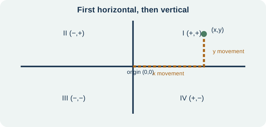
Coordinates may carry physical units. A map point $(3.0\ \mathrm{km},-2.0\ \mathrm{km})$ records two signed distances relative to an origin and oriented axes. Both components must use compatible length units before a Euclidean distance formula is applied. A graph of unlike quantities can use different axis units, but its geometric slope then has contextual units. Axis scale and units belong to the mathematical description.

Encode displacement with coordinate differences

From $A(x_1,y_1)$ to $B(x_2,y_2)$, horizontal change is $\Delta x=x_2-x_1$ and vertical change is $\Delta y=y_2-y_1$. The Greek capital delta denotes finite change. Endpoint minus starting point preserves direction. Either component may be positive, negative, or zero. The ordered pair $(\Delta x,\Delta y)$ is the displacement from $A$ to $B$.

Reversing direction negates both components. The displacement from $B$ to $A$ is $(x_1-x_2,y_1-y_2)=(-\Delta x,-\Delta y)$. Its magnitude is unchanged even though direction reverses. Reversing only one component would describe a reflection rather than the reverse segment. Consistent endpoint order matters.

For $A=(-3,2)$ and $B=(5,8)$, the displacement is $(5-(-3),8-2)=(8,6)$. This means eight coordinate units right and six units up. From $B$ back to $A$, displacement is $(-8,-6)$. A quick sketch should agree with these signs. Displacement is directed, while distance will be nonnegative.

Derive the distance formula from the Pythagorean theorem

Horizontal and vertical coordinate changes form perpendicular legs of a right triangle whose hypotenuse is segment $AB$. The Pythagorean theorem gives $AB^2=(\Delta x)^2+(\Delta y)^2$. Taking the nonnegative square root gives $AB=\sqrt{(x_2-x_1)^2+(y_2-y_1)^2}$. Squaring removes the signs of directed components. Distance is therefore independent of travel direction.

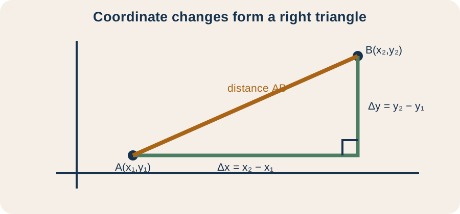
For $A=(-3,2)$ and $B=(5,8)$, distance is $\sqrt{8^2+6^2}=\sqrt{64+36}=\sqrt{100}=10$. If coordinates are measured in centimeters, the answer is $10\ \mathrm{cm}$. The squared terms temporarily have units $\mathrm{cm^2}$, and the square root returns linear units. Dimensional analysis agrees with geometric meaning. The result is nonnegative and independent of endpoint order.

Exact radicals should be preserved when they do not simplify. A distance $\sqrt{17}$ communicates exact structure, while a decimal such as $4.123$ is an approximation. Approximate only when context requires it and label the result with $\approx$. The distance formula is also a strong congruence tool because equal squared distances imply equal positive distances. Squared comparisons can avoid unnecessary radicals.

Derive midpoint and section formulas

The midpoint of $A(x_1,y_1)$ and $B(x_2,y_2)$ is $M=\left(\frac{x_1+x_2}{2},\frac{y_1+y_2}{2}\right)$. Each coordinate is the arithmetic mean of corresponding endpoint coordinates. Starting at $A$, moving half the displacement gives $x_1+\frac{x_2-x_1}{2}=\frac{x_1+x_2}{2}$. The same reasoning applies vertically. Thus the formula locates the point halfway along both coordinate changes.

For $A=(-3,2)$ and $B=(5,8)$, midpoint is $\left(\frac{-3+5}{2},\frac{2+8}{2}\right)=(1,5)$. Displacement from $A$ to $M$ is $(4,3)$, and displacement from $M$ to $B$ is also $(4,3)$. Equal displacement confirms the bisection. Distance checks give $AM=MB=5$. Both coordinate and metric tests support the same conclusion.

A point dividing $AB$ in fraction $t$ of the way from $A$ to $B$ has coordinates $P=(1-t)A+tB$. Componentwise, $P=(x_1+t(x_2-x_1),y_1+t(y_2-y_1))$. Values $0<t<1$ lie inside the segment, while values outside that range extend beyond an endpoint. The midpoint corresponds to $t=\frac{1}{2}$. This vector-like formula generalizes averaging to any division ratio.

Interpret slope as directional rate

For a nonvertical line through two points, slope is $m=\frac{y_2-y_1}{x_2-x_1}=\frac{\Delta y}{\Delta x}$. The numerator is vertical change and the denominator is horizontal change. Slope describes output change per horizontal input change. Its sign records whether the line rises or falls from left to right. Its magnitude records steepness relative to axis scales.

Reversing both point orders leaves slope unchanged. Multiplying numerator and denominator by negative one preserves the quotient. A horizontal line has $\Delta y=0$ and slope zero. A vertical line has $\Delta x=0$, so its slope is undefined rather than zero. This distinction is essential for perpendicularity and line equations.

Slope can have units. On a position-versus-time graph, slope may be $5.0\ \frac{\mathrm m}{\mathrm s}$. On an ordinary geometric coordinate plane where both axes use meters, units cancel and slope is dimensionless. Visual angle depends on axis scaling, so slope should be computed from coordinates. A line that looks steep on a distorted graph may have a modest numerical rate.

Write line equations from geometric information

Point-slope form is $y-y_1=m(x-x_1)$. It states that any point $(x,y)$ on the line has the same slope relative to fixed point $(x_1,y_1)$. The parentheses preserve the coordinate differences. This form is especially useful when a point and slope are known. Substitution of the fixed point makes both sides zero.

Slope-intercept form is $y=mx+b$, where $m$ is slope and $b$ is the $y$-intercept. Starting from point-slope form, expand and solve for $y$. The intercept is the output when $x=0$. It may not be geometrically relevant if the plotted domain excludes zero. Line form should serve the available information and intended interpretation.

Vertical lines cannot be written as $y=mx+b$ because their slope is undefined. A vertical line through horizontal coordinate $h$ has equation $x=h$. A horizontal line through vertical coordinate $k$ has equation $y=k$. Standard form $Ax+By=C$ can represent both cases. No one line form is universally best.

Test parallel and perpendicular lines

Distinct nonvertical lines are parallel when their slopes are equal. Equal slope means their direction vectors are scalar multiples. Vertical lines are parallel to other vertical lines. Coincident lines share all points and should be distinguished from separate parallel lines when context requires. Intercepts help determine whether equal-slope lines are distinct.

Nonvertical, nonhorizontal lines are perpendicular when their slopes multiply to $-1$. Equivalently, one slope is the negative reciprocal of the other. A line of slope $\frac{2}{3}$ is perpendicular to a line of slope $-\frac{3}{2}$. Horizontal and vertical lines provide the remaining perpendicular case. The product test cannot be applied when one slope is undefined.

Direction vectors provide a unified test. Vectors $(a,b)$ and $(c,d)$ are perpendicular when their dot product $ac+bd$ equals zero. A vertical direction $(0,1)$ and horizontal direction $(1,0)$ have dot product zero. This method avoids special slope cases. It also extends naturally to higher dimensions.

Classify figures with multiple necessary properties

Coordinate classification requires sufficient evidence. A parallelogram can be established by showing both pairs of opposite sides are parallel or by showing diagonals share a midpoint. A rectangle requires a parallelogram with one right angle or equivalent evidence. A rhombus requires a parallelogram with equal side lengths. A square must satisfy both rectangle and rhombus conditions.

Consider $A(0,0)$, $B(4,1)$, $C(3,5)$, and $D(-1,4)$. Side displacement vectors are $\overrightarrow{AB}=(4,1)$, $\overrightarrow{BC}=(-1,4)$, $\overrightarrow{CD}=(-4,-1)$, and $\overrightarrow{DA}=(1,-4)$. Opposite vectors are negatives, so opposite sides are parallel and equal. Adjacent dot product is $(4)(-1)+(1)(4)=0$, proving a right angle. Adjacent lengths both equal $\sqrt{17}$, so the figure is a square.

A drawing alone cannot prove this classification because plotting scales and hand accuracy may mislead. Equal sides alone could describe a rhombus rather than a square. Perpendicular diagonals alone are also insufficient in general. List the theorem connecting computed properties to the classification. Coordinate evidence must be interpreted through geometric definitions.

Translate distance conditions into loci

A locus is the set of all points satisfying a geometric condition. Points at fixed distance $r$ from center $(h,k)$ form a circle. Applying the distance formula gives $\sqrt{(x-h)^2+(y-k)^2}=r$. Squaring both nonnegative sides yields $(x-h)^2+(y-k)^2=r^2$. The equation encodes center and radius directly.

For center $(2,-1)$ and radius $4$, the circle equation is $(x-2)^2+(y+1)^2=16$. The plus sign inside the second square appears because $y-(-1)=y+1$. Substituting center gives zero on the left, not sixteen, because the center is not on a positive-radius circle. Substituting $(6,-1)$ gives sixteen and verifies one point. Sign checks should follow coordinate differences rather than visual memory.

The perpendicular bisector of segment $AB$ is the locus of points equidistant from $A$ and $B$. Set squared distances equal to avoid square roots. Quadratic terms in $x^2$ and $y^2$ cancel, leaving a linear equation. The resulting line passes through the midpoint and is perpendicular to $AB$. Algebra reproduces the classical construction.

Use coordinate geometry for intersections

An intersection point satisfies the equations of every object meeting there. Two nonparallel lines produce a system of two linear equations. Solving the system finds their common coordinate pair. Parallel distinct lines yield no solution, while coincident lines yield infinitely many. Algebraic solution counts match geometric intersection counts.

A line and circle can have zero, one, or two intersection points. Substitute the line equation into the circle equation to obtain a quadratic. A negative discriminant gives no real intersection, zero gives tangency, and positive gives two crossings. The discriminant converts geometric contact into algebraic cases. Substitution results should be returned to both original equations.

Two circles can likewise be compared by subtracting their equations. Squared terms cancel and often produce a line containing possible intersection points. Solving that line with one circle completes the calculation. The method is an example of eliminating shared nonlinear structure. Coordinate geometry turns construction questions into systems.

Describe translations, reflections, and rotations

A translation by vector $(a,b)$ sends $(x,y)$ to $(x+a,y+b)$. Every point receives the same displacement, so distances, angles, parallelism, and orientation are preserved. Translation moves the origin unless $(a,b)=(0,0)$. It is an affine transformation rather than a linear transformation in ordinary two-dimensional vector coordinates. Geometry remains congruent.

Common reflections have simple coordinate rules. Reflection across the $x$-axis sends $(x,y)$ to $(x,-y)$, while reflection across the $y$-axis sends it to $(-x,y)$. Reflection across $y=x$ swaps coordinates, producing $(y,x)$. Each rule can be verified by equal perpendicular distance to the mirror line. Reflections reverse orientation while preserving length and angle.

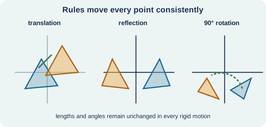
A counterclockwise rotation by $90^{\circ}$ about the origin sends $(x,y)$ to $(-y,x)$. Applying the rule twice gives $(-x,-y)$, a $180^{\circ}$ rotation. Four applications restore the original point. Rotations about another center can be performed by translating the center to the origin, rotating, and translating back. Composition order must be preserved.

Choose coordinates strategically for proof

Coordinate proof begins by placing a general figure conveniently. A segment of length $2a$ can be placed with endpoints $(-a,0)$ and $(a,0)$ so its midpoint is the origin. A rectangle may use $(0,0)$, $(w,0)$, $(w,h)$, and $(0,h)$. The variables retain general side lengths. Symmetry reduces algebra without assuming a special square.

Overly special placement can invalidate generality. Assigning equal horizontal and vertical side lengths assumes a rectangle is a square. Placing a diagonal on an axis may be valid only if every allowed figure can be moved there by a rigid transformation. State why the placement loses no relevant generality. Coordinates should encode known conditions and nothing more.

After placement, translate the desired property into a calculable test. Use distance for congruence, midpoint for bisection, slope or dot product for direction, and systems for intersection. Simplify symbolically rather than testing a single numerical example. Finish by naming the geometric theorem that the algebra establishes. A coordinate proof needs a conclusion, not only calculations.

Extend coordinates to three dimensions

In three dimensions, a point has coordinates $(x,y,z)$. Displacement from $A$ to $B$ is $(x_2-x_1,y_2-y_1,z_2-z_1)$. Distance becomes $\sqrt{(x_2-x_1)^2+(y_2-y_1)^2+(z_2-z_1)^2}$. The formula follows by applying the Pythagorean theorem twice. Midpoint averages all three coordinate pairs.

Lines in space are conveniently described parametrically as $\mathbf r=\mathbf r_0+t\mathbf v$. The vector $\mathbf r_0$ locates one point and $\mathbf v$ supplies direction. Planes can be described using a normal vector. Dot products test perpendicularity without relying on slope. The two-dimensional concepts generalize through vectors.

Units remain essential. If horizontal coordinates are kilometers but elevation is meters, convert before computing Euclidean distance. Otherwise the numerical components do not share a common scale. Geographic coordinates on a curved Earth also require models beyond a flat Cartesian plane over large regions. Coordinate formulas inherit the assumptions of the chosen geometry.

Verify coordinate calculations systematically

Begin with a labeled sketch and a coordinate inventory. Check point order, axis orientation, scale, and units. Predict signs of coordinate changes and rough magnitude of distances. Choose a formula or theorem tied to the requested property. Write differences before squaring or dividing.

Next calculate exactly when possible. Preserve consistent endpoint order in both slope differences. Keep radicals and fractions until approximation is useful. Check denominators for zero before using slope. Substitute candidate points into equations.

Finally return to geometry. Confirm distance is nonnegative, midpoint lies halfway, slopes match visible direction under the actual scale, and transformation preserves intended invariants. Use an alternative test such as dot product versus slope when possible. State the geometric conclusion in words. Independent checks make a coordinate proof reliable.

Diagnose common mistakes

One mistake reverses only one coordinate difference in slope, creating the wrong sign. Choose an ordered pair of endpoints and use it consistently. Another calls vertical slope zero. Zero belongs to horizontal change in output, while vertical slope is undefined because horizontal change is zero. Draw direction vectors to reinforce the distinction.

Distance errors often omit a square, forget parentheses around negative differences, or use the Manhattan sum $|\Delta x|+|\Delta y|$ instead of Euclidean distance. Write the right triangle and square complete differences. Midpoint errors divide coordinate differences rather than coordinate sums by two. Derive midpoint from starting point plus half displacement when uncertain. Meaning reconstructs the formulas.

Proof errors arise from insufficient properties or special diagrams. Equal diagonals alone do not prove a quadrilateral is a rectangle without additional structure. A plotted square-looking figure is not evidence of equal lengths or right angles. State definitions and theorems explicitly. Coordinate geometry replaces visual guessing with verifiable relationships.

Practice calculation, classification, and proof

For $A=(-3,2)$ and $B=(5,8)$, find displacement, distance, midpoint, and slope. Attach units if coordinates are measured in meters. Verify the midpoint by comparing two displacement vectors. Write the perpendicular-bisector equation by equating squared distances. Check that the midpoint satisfies it.

Write the circle centered at $(2,-1)$ with radius $4$. Identify its leftmost, rightmost, highest, and lowest points. Determine whether $(5,1)$ lies inside, on, or outside the circle using squared distance. Explain the sign in $y+1$. Describe the result geometrically.

Let $A(0,0)$, $B(6,0)$, $C(8,4)$, and $D(2,4)$. Classify the quadrilateral using slopes or vectors and side lengths. Find diagonal midpoints. Decide whether it is a rectangle, rhombus, or square in addition to its broadest classification. Provide sufficient evidence and explain why appearance alone is inadequate.

Solutions and reasoning

For the first problem, displacement is $(8,6)$, distance is $10$ units, midpoint is $(1,5)$, and slope is $\frac{6}{8}=\frac{3}{4}$. Equal-distance equation is $(x+3)^2+(y-2)^2=(x-5)^2+(y-8)^2$. Simplification gives $4x+3y=19$. The midpoint satisfies $4(1)+3(5)=19$. Its direction has slope $-\frac{4}{3}$, the negative reciprocal of $\frac{3}{4}$.

The circle equation is $(x-2)^2+(y+1)^2=16$. Extreme points are $(-2,-1)$, $(6,-1)$, $(2,3)$, and $(2,-5)$. For $(5,1)$, squared distance to center is $(3)^2+(2)^2=13$. Since $13<16$, the point lies inside. The plus sign comes from subtracting center coordinate negative one.

Side vectors are $(6,0)$, $(2,4)$, $(-6,0)$, and $(-2,-4)$, so opposite sides are parallel and the figure is a parallelogram. Adjacent dot product is $(6)(2)+(0)(4)=12$, so sides are not perpendicular. Side lengths are $6$ and $\sqrt{20}$, so they are not all equal. Diagonal midpoints are both $(4,2)$, confirming bisection. The figure is neither rectangle, rhombus, nor square.

Carry coordinate reasoning into vectors and analytic geometry

Coordinate geometry joins algebra and geometry through a repeatable translation process. Differences encode displacement, squares encode distance, ratios encode direction, averages encode bisection, and equations encode loci. Each formula can be rebuilt from these meanings. Exact calculation supports claims that a drawing can only suggest. Units and scale keep the results connected to applications.

Vectors formalize displacement and provide dot products, projections, and transformations. Linear algebra represents coordinate transformations with matrices. Analytic geometry extends circles to conic sections and surfaces. Calculus studies slopes and accumulated change on coordinate graphs. The coordinate plane is a foundation rather than an endpoint.

When solving a coordinate problem, begin with the geometric condition and choose coordinates that preserve its generality. Translate the condition into a formula, compute carefully, and interpret the algebraic result geometrically. Verify through a second representation whenever possible. That cycle turns coordinates into a proof language rather than a plotting convenience. Every algebraic conclusion should return to the geometry that motivated it.