Covalent Bonding

Covalent bonding occurs when electron density is distributed across two or more atomic centers in a stabilizing way. The familiar phrase “atoms share electrons” is a useful starting image, but it can sound as though stationary particles are divided by agreement. Electrons instead occupy quantum states that extend through the bonded region. Their distribution changes electron–nucleus attraction, electron–electron repulsion, nuclear repulsion, and electron kinetic energy. A stable bond appears when the complete interacting system has an energy minimum at finite separation.

Covalent bonds range from nearly equal sharing to strongly polarized sharing. They can be localized mainly between two atoms or delocalized across a larger framework. Single, double, and triple lines in Lewis structures summarize electron-pair bookkeeping but do not display an exact electron-density map. Orbital models explain direction, symmetry, and energy more deeply. Experimental bond lengths, energies, spectra, and charge distributions test every representation.

This article coordinates three levels of description. Lewis structures organize valence electrons and connectivity. Orbital-overlap models explain sigma and pi bonding, while molecular-orbital ideas explain bonding and antibonding states. Geometry and polarity connect microscopic electron distribution to molecular behavior. A reliable explanation uses the simplest model that answers the question while stating its limits.

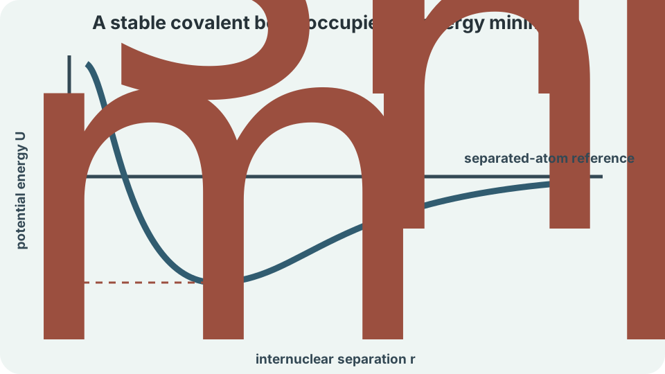
A covalent bond is an energy minimum

Imagine two atoms approaching from a very large separation. Attractive interactions between each nucleus and the other atom’s electrons can lower potential energy. Nuclear repulsion and electron–electron repulsion oppose that stabilization. Quantum restrictions also raise energy when electron clouds are compressed into unfavorable states. The combined energy can form a well.

The distance at the bottom of the well is the equilibrium bond length $r_e$. The subscript $e$ labels equilibrium. Small stretching or compression raises potential energy, producing a restoring force. At distances much larger than $r_e$, the atoms approach separated fragments. At distances much smaller than $r_e$, repulsion rises steeply.

Force is related to potential energy by $F=-\frac{dU}{dr}$. The symbol $F$ is radial force, $U$ is potential energy, $r$ is internuclear separation, and the derivative describes the curve’s slope. At the minimum, $\frac{dU}{dr}=0$, so net radial force is zero. Individual attractive and repulsive contributions still exist there. Their sum balances at equilibrium.

Shared density stabilizes the internuclear region

Electron density placed between two positive nuclei is attracted to both. This can lower electron–nucleus potential energy relative to separated atoms. The density also partially screens nuclear repulsion. Stabilization is not guaranteed because electron repulsion and kinetic-energy changes must be included. Favorable total energy, not sharing by itself, defines bonding.

The simplest covalent bond is found in $\mathrm{H_2}$. Each hydrogen contributes one electron, and the pair occupies a bonding molecular state. Increased density appears between the nuclei compared with separated atoms. The equilibrium molecule lies lower in energy than two isolated ground-state hydrogen atoms. Energy must be supplied to dissociate it.

Electron density is a probability distribution rather than a path followed by an electron. A cloud drawing shows where detection is likely over repeated measurements. It does not give a hard surface. Bond diagrams deliberately compress three-dimensional quantum information. Their meaning must be taught rather than inferred from artistic shape.

Orbital overlap introduces direction and symmetry

Atomic orbitals are mathematical wavefunctions associated with electron states in isolated-atom models. When atoms interact, compatible orbitals can combine. Constructive combination increases wavefunction amplitude in some regions. Destructive combination creates reduced amplitude or a node. The resulting molecular states belong to the whole molecule.

Effective overlap requires compatible symmetry, energy, and spatial orientation. Two orbitals pointing toward each other can overlap strongly along the internuclear axis. Orbitals with incompatible orientation may overlap weakly or cancel by symmetry. Greater overlap often increases separation between bonding and antibonding energy levels. Distance cannot become arbitrarily small because repulsive contributions then dominate.

Hybrid orbital language reorganizes atomic-orbital functions to match local geometry. The labels $\mathrm{sp}$, $\mathrm{sp^2}$, and $\mathrm{sp^3}$ describe common combinations in a valence-bond model. They help explain linear, trigonal-planar, and tetrahedral bond directions. Hybridization is a model representation rather than a physical mixing event observed in time. Molecular-orbital descriptions can represent the same molecule without assigning localized hybrids.

Sigma bonds concentrate density along the axis

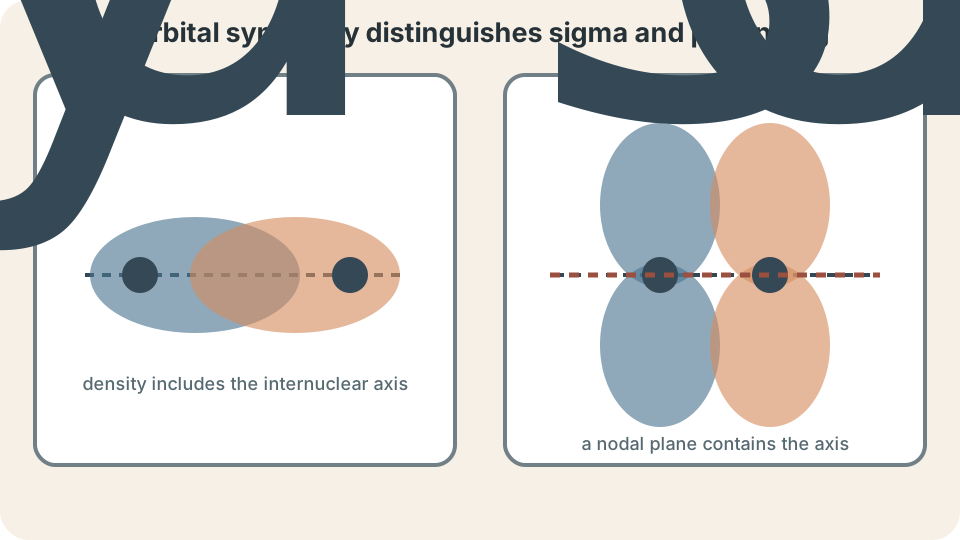
A sigma bond has cylindrical symmetry around the internuclear axis in the idealized model. The Greek letter $\sigma$, pronounced “sigma,” labels this symmetry. Head-on overlap of two $s$ orbitals, an $s$ and a directed orbital, or two directed orbitals can create sigma bonding. Rotation around the axis leaves the density pattern unchanged. Every ordinary single bond contains one sigma framework.

Sigma bonding density lies directly between the nuclei. This usually permits stronger overlap than side-by-side overlap of comparable orbitals. A corresponding sigma-star state, written $\sigma^*$, is antibonding. The star marks an orbital with destabilizing character relative to the associated bonding combination. Occupying antibonding states reduces net bond order.

Single bonds often allow rotation because the sigma overlap survives as one bonded group turns around the axis. Rotation may still face energy barriers from steric crowding, conjugation, or partial double-bond character. “Single bonds rotate freely” is therefore an approximation. The local electronic environment determines the actual rotational energy profile. Conformational analysis measures those energy changes as the rotation angle varies.

Pi bonds add side-by-side overlap

A pi bond forms from side-by-side overlap of parallel orbitals, commonly unhybridized $p$ orbitals. The Greek letter $\pi$, pronounced “pie,” labels this symmetry. Bonding density occupies regions above and below the internuclear axis. A nodal plane passes through the axis in the ideal picture. The sign of a wavefunction lobe is phase, not electric charge.

A double bond contains one sigma bond and one pi bond in a localized valence-bond description. A triple bond contains one sigma bond and two mutually perpendicular pi bonds. The first connection between two atoms is sigma because head-on overlap defines the axis. Additional localized bond components use pi symmetry. Counting sigma and pi components is not the same as counting electron pairs anywhere in the molecule.

Pi overlap depends strongly on parallel alignment. Twisting one group relative to another reduces overlap and raises energy. This restricts rotation around many double bonds and permits stable geometric isomers. Breaking only the pi component can allow reorientation in a reaction pathway. The sigma framework can remain connected during that step.

Bond order connects electrons to strength

In a localized Lewis description, single, double, and triple bonds have bond orders one, two, and three. Higher bond order commonly means more density concentrated in bonding regions between the same pair of atom types. Comparable higher-order bonds are generally shorter and stronger. The qualifier “comparable” controls the trend. Atomic size, charge, environment, and delocalization also matter.

In a basic molecular-orbital description, bond order is $\frac{N_b-N_a}{2}$. The symbol $N_b$ is the number of electrons in bonding orbitals, and $N_a$ is the number in antibonding orbitals. The subtraction measures net stabilizing occupation. Division by two reflects two electrons per ordinary bonding pair. A positive bond order supports net bonding in this simplified model.

Resonance can produce fractional average bond orders. Benzene’s six carbon–carbon bonds are equivalent rather than alternating as fixed single and double bonds. Nitrate has three equivalent nitrogen–oxygen bonds with average order $\frac{4}{3}$ in a simple contributor average. Fractional order represents delocalized character. It does not mean a bond changes back and forth between integer values.

Lewis structures are disciplined bookkeeping

A Lewis structure counts valence electrons, connects atoms, and assigns bonding and nonbonding pairs. Each ordinary line represents two electrons. Dots represent nonbonding electrons. Formal charge evaluates an atom with $\mathrm{FC}=V-N-\frac{B}{2}$. The symbols represent neutral valence count, nonbonding electrons, and bonding electrons respectively.

The octet rule predicts many stable arrangements for second-period main-group atoms. It is a pattern, not the cause of covalent attraction. Hydrogen follows a duet because only the $1s$ shell is available. Boron compounds can be electron deficient, and odd-electron species cannot give every atom an octet. Heavier atoms and transition metals require broader models.

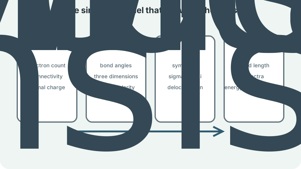
Lewis structures are strongest at connectivity, electron counting, and identifying possible resonance. They are weaker at predicting exact geometry, energy, magnetism, and delocalized electron density. VSEPR adds a geometry model. Molecular-orbital theory adds whole-molecule electronic states. No one diagram should be asked to answer every question.

Coordinate covalent bonds have the same final status

A coordinate covalent bond is drawn when both electrons in a new shared pair originate from one participant’s lone pair. A Lewis base donates the pair, and a Lewis acid accepts it. A curved arrow can show pair movement from donor to acceptor. This describes bond formation bookkeeping. After formation, the shared pair belongs to the bonded system.

Ammonia can donate a lone pair to a proton to form ammonium. The new nitrogen–hydrogen connection may be described as coordinate during formation. In the resulting ideal ammonium ion, all four nitrogen–hydrogen bonds are equivalent. The molecule does not permanently label which bond was donated. Formation history and final structure are different descriptions.

Metal–ligand bonds are often introduced with coordinate covalent language. Ligands donate electron density into available metal-centered states, and back-donation may occur in the opposite direction. Real bonding can include electrostatic and covalent contributions. The simple arrow begins an analysis rather than completes it. Spectroscopic and structural evidence refine the model.

Unequal sharing creates polar covalent bonds

Different atoms often attract bonding density unequally. Electronegativity summarizes the relative tendency to draw shared density. The more electronegative end becomes partially negative, written $\delta-$, while the other becomes $\delta+$. The Greek delta indicates partial rather than full ionic charge. The molecule can remain neutral overall.

A bond dipole has direction and magnitude. In the simple relationship $\mu=qr$, $\mu$ is dipole moment, $q$ is separated charge magnitude, and $r$ is separation. Molecular dipole moment is a vector sum over the whole geometry. Polar bonds can cancel in a symmetric molecule. Carbon dioxide is a standard example.

Ionic and covalent descriptions form a continuum. A highly polar bond can have substantial ionic character without belonging to a simple ionic lattice. Environmental fields and neighboring groups shift electron density. Electronegativity cutoffs are teaching conventions. Evidence determines which model is productive.

Resonance represents delocalized covalency

Resonance contributors preserve atomic connectivity while changing electron placement. They are connected by a resonance arrow rather than a reaction or equilibrium arrow. The real structure is a delocalized hybrid. It does not switch rapidly among drawings. Equivalent contributors contribute equally by symmetry.

Delocalization can spread bonding and charge across three or more atoms. This often lowers energy relative to an artificially localized electron arrangement. Equal measured bond lengths can support the model. Spectroscopy and computation provide additional evidence. Formal charge helps rank unequal contributors.

Conjugation requires compatible adjacent orbitals. Planarity often improves continuous overlap, while twisting can interrupt it. Delocalization can restrict rotation and change reactivity. Amide bonds show partial double-bond character because a nitrogen lone pair interacts with a neighboring carbonyl system. Structure, energy, and motion are connected.

Molecular geometry emerges from electron distribution

VSEPR predicts local shape by arranging electron domains around a central atom. Bonding groups and lone pairs occupy regions whose repulsions influence geometry. Multiple bonds count as one domain for basic geometry but can exert a larger spatial influence. Electron-domain geometry includes lone pairs. Molecular geometry names atom positions.

Geometry determines bond angles and vector relationships. Tetrahedral methane has angles near $109.5^\circ$. Trigonal-planar environments have ideal angles near $120^\circ$, and linear environments near $180^\circ$. Real angles deviate because domains differ. Measured geometry tests the model.

Orbital symmetry and energetic optimization offer deeper explanations than literal electron-pair balloons. VSEPR is valuable because it predicts many foundational shapes quickly. Hybridization can organize directional bonding in a localized model. Molecular orbitals describe delocalized states over the full framework. Choose the level that matches the evidence and task.

Covalent substances have diverse properties

Small molecular substances consist of strong internal covalent bonds and weaker attractions between molecules. Melting or boiling usually rearranges intermolecular contacts rather than breaking the molecular framework. Their phase-change temperatures can therefore be modest. Polarity, hydrogen bonding, dispersion, and shape control the comparison. The word “covalent” alone does not predict a boiling point.

Network covalent solids contain bonds extending through a large structure. Diamond connects each carbon in a three-dimensional network. Graphite contains strong in-plane networks with weaker interactions between layers. Their different topology produces different hardness and conductivity. Composition alone does not determine property.

Polymers contain long covalently connected chains whose intermolecular organization varies. Cross-linking can stiffen a material and reduce chain mobility. Crystallinity, branching, chain length, and intermolecular attraction influence strength and melting behavior. A single repeat-unit drawing omits important higher-scale structure. Materials reasoning must connect several length scales.

Experimental evidence tests bond models

Diffraction methods estimate atomic positions and bond lengths. Equivalent lengths can reveal symmetry or delocalization. Vibrational spectroscopy probes energy changes associated with bond stretching and bending. Higher stretching frequency often indicates greater effective stiffness for comparable reduced masses. Mass must be considered alongside bond strength.

Bond dissociation energy measures an energy required for a specified gas-phase bond-breaking process. It depends on the molecule and the fragments produced. Average bond energies are approximations collected across related compounds. They can estimate reaction enthalpy but are not exact constants for every bond label. The written process defines the quantity.

Photoelectron and absorption spectroscopy probe electronic energy levels. Magnetic behavior can reveal unpaired electrons that a simple Lewis structure misses. Electron-density calculations and scattering evidence refine charge distribution. A scientific model earns confidence by coordinating different measurements. Attractive pictures alone are not evidence.

A reliable covalent-bonding workflow

First count valence electrons and establish connectivity. Draw a Lewis structure, calculate formal charges, and identify resonance contributors. Confirm the total electron count and net charge. State any octet exception. This creates an auditable bookkeeping foundation.

Second determine three-dimensional geometry and likely orbital relationships. Identify sigma and pi components where useful. Decide whether conjugation or resonance delocalizes electron density. Mark bond dipoles and add them as vectors for molecular polarity. Explain the limitations of each model used.

Third connect the bonding model to a measured or predicted property. Use bond order and atom identity for cautious length or strength comparisons. Use intermolecular interactions for phase properties of molecular substances. Use network topology for extended solids. Name the evidence that could test the conclusion.

Retrieval practice and synthesis

Explain why a carbon–carbon double bond resists rotation more than a carbon–carbon single bond. Identify its sigma and pi components. Describe how twisting reduces side-by-side orbital overlap. State that the energy barrier depends on environment. Avoid saying two atoms are connected by two rigid sticks.

Compare $\mathrm{N_2}$ and $\mathrm{O_2}$ using bond order and molecular-orbital evidence. Nitrogen has a strong triple-bond description and a high dissociation energy. Oxygen has bond order two in the elementary molecular-orbital model and contains unpaired electrons. Those unpaired electrons explain paramagnetism that a simple Lewis drawing hides. Different evidence selects different model depth.

Choose a molecule with resonance and construct a claim–evidence–reasoning explanation. The claim should identify equal or intermediate bond character. The evidence should include valid contributors and measured or predicted bond lengths. The reasoning should connect delocalized density to average bond order. End by stating why the contributors are not rapidly interconverting species.