Linear Equations Express Balance

An equation states that two expressions have the same value. Solving means finding every input that makes that statement true. The central principle is not moving symbols but preserving a solution set through reversible transformations. This perspective explains standard procedures and exposes their limits. It also connects equations to graphs, units, parameters, and physical models.

Read equality as a relationship

The equals sign does not mean “now calculate the answer.” It asserts that the expression on the left and the expression on the right represent the same quantity. Neither side has priority. Either side can contain variables, operations, or measured quantities. Reversing the sides leaves the relationship unchanged. This symmetry is one of equality’s defining properties.

This relational meaning differs from an arithmetic worksheet pattern. In $3+4=7$, the right side happens to display a computed value. In $3+4=5+2$, both sides are expressions and the equality remains true. In $2x+1=9$, truth depends on the value assigned to $x$. Algebra studies exactly which assignments make such relationships true.

The solution set is the collection of all values that satisfy an equation. Some equations have one solution, some have none, and some are true for every allowed input. Solving must preserve all satisfying values and exclude all nonsatisfying values. A sequence of steps is successful only when its final statement has the same solution set as the original. This criterion is more precise than saying the variable has merely been isolated.

Use reversible properties of equality

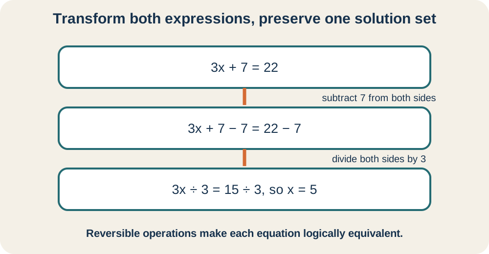
If $A=B$, adding the same quantity $C$ gives $A+C=B+C$. Subtracting is addition of an opposite, so it obeys the same property. Multiplying both sides by the same quantity also preserves equality. Division is multiplication by a reciprocal and therefore requires a nonzero divisor. These operations justify most linear-equation transformations.

Reversibility is what preserves the complete solution set. If two is added to both sides, subtracting two reverses the step. If both sides are multiplied by nonzero five, division by five reverses it. Each equation implies the one before and after it. The equations are logically equivalent rather than merely similar-looking.

Some operations preserve truth in only one direction. Squaring equal expressions produces equal squares, but equal squares can come from opposite original values. From $x=-2$ one may infer $x^2=4$, yet $x^2=4$ also admits $x=2$. Squaring can therefore introduce an extraneous solution. Linear solving is unusually clean because addition and nonzero scaling are reversible.

Replace “moving terms” with named operations

Students are often told that a term crosses the equals sign and changes sign. This shorthand can predict a written result but hides the equality-preserving action. In $5x-7=18$, the negative seven does not travel. Adding seven to both sides gives $5x-7+7=18+7$. Additive inverses then simplify the left side.

The coefficient five does not jump under the other side either. Divide both sides by five to obtain $\frac{5x}{5}=\frac{25}{5}$. Nonzero common factors simplify, producing $x=5$. Naming the operation explains both why the step works and why division by zero is forbidden. The narrative remains reliable when expressions become more complicated.

Good notation should show enough intermediate structure to audit the reasoning. Writing one equality per line keeps the relationship visible. Aligning equals signs helps a reader compare transformations. Mental arithmetic may simplify constants, but hidden sign changes deserve an explicit line. Clarity is part of correctness because it makes unsupported transformations detectable.

Solve while narrating the structure

Consider $3(2x-1)+4=5x+9$. Distribution gives $6x-3+4=5x+9$, and combining like terms gives $6x+1=5x+9$. Subtracting $5x$ from both sides gives $x+1=9$. Subtracting one from both sides gives $x=8$. Each step preserves the solution set.

Verification returns to the original equation rather than the final simplified one. Substituting eight into the left side gives $3(16-1)+4=49$. Substituting eight into the right side gives $40+9=49$. Both expressions produce the same value. This check can catch distribution, sign, and arithmetic errors.

Verification is evidence, not a replacement for reasoning. Testing one candidate proves that candidate works but does not always prove no others exist. The reversible linear steps establish equivalence and therefore completeness. The substitution check confirms the resulting candidate in the original domain. Together they provide stronger support than either alone.

Clear numerical denominators legally

Fractions do not change the balance principle. For $\frac{x-1}{3}+\frac{x+2}{2}=5$, the least common denominator is six. Multiply every term on both sides by six. This gives $2(x-1)+3(x+2)=30$. Simplification then yields $5x+4=30$ and $x=\frac{26}{5}$.

The phrase “every term” matters. Multiplying only the visible fractions changes the equation because the right-side five would remain unscaled. Parentheses preserve complete numerators during distribution. A horizontal fraction bar groups its entire numerator and denominator. Reading that grouping correctly prevents partial multiplication.

When a denominator contains a variable, record domain restrictions before clearing it. The equation $\frac{2}{x-1}=3$ requires $x\ne1$. Multiplying by $x-1$ gives $2=3(x-1)$ and candidate $x=\frac{5}{3}$. That value respects the restriction and verifies in the original equation. An excluded value could never be restored by later simplification.

Classify one, no, or infinitely many solutions

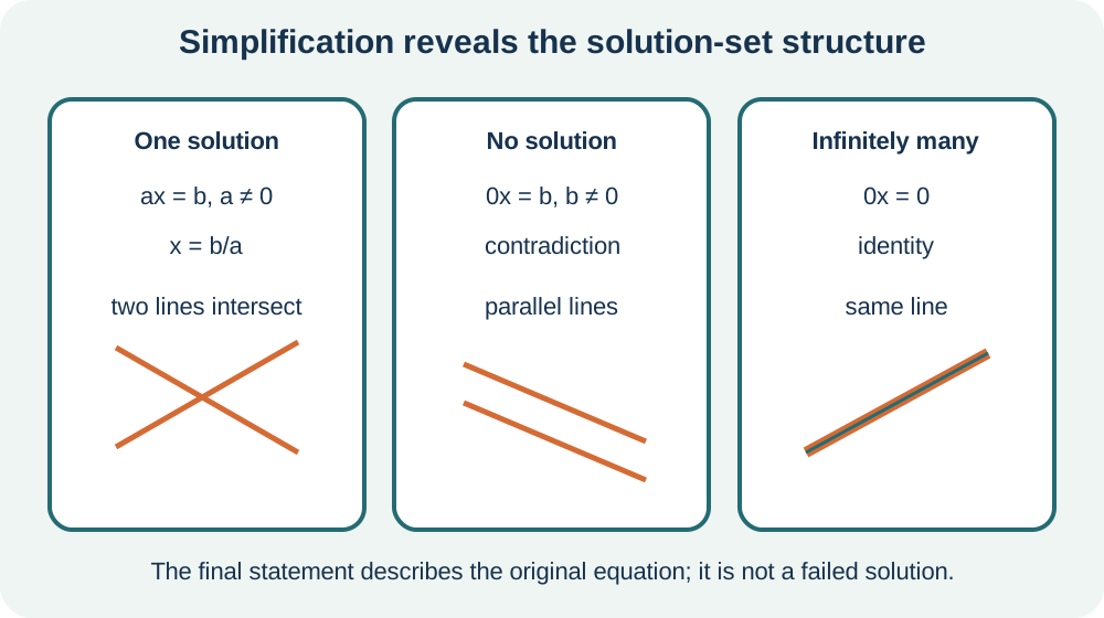
After collecting terms, a one-variable linear equation can be reduced to $ax=b$. If $a\ne0$, division gives the unique solution $x=\frac{b}{a}$. If $a=0$ and $b\ne0$, the equation becomes a contradiction such as $0=3$. If both are zero, it becomes an identity such as $0=0$. These outcomes exhaust the linear possibilities.

For $2(x+1)=2x+2$, expansion gives $2x+2=2x+2$. Subtracting $2x$ from both sides produces $2=2$. This true statement is independent of $x$, so every real input satisfies the original equation. The disappearance of the variable reveals an identity rather than a failed calculation. Any original domain restrictions would still limit the otherwise universal solution set.

For $2(x+1)=2x+3$, expansion and subtraction produce $2=3$. No value of $x$ can make this false statement true. The original equation therefore has no solution. A contradiction is a valid structural conclusion. It should not be repaired by inventing another algebraic step.

Connect algebraic outcomes to graphs

An equation can be interpreted as asking where two functions have equal outputs. For $2x+1=7-x$, graph $y=2x+1$ and $y=7-x$. A solution is an input where the graphs share the same point. Solving algebraically gives $3x=6$ and $x=2$. Both graph outputs equal five there.

Two nonparallel lines intersect exactly once. Their unequal slopes create one shared point, matching a one-solution equation. Distinct parallel lines never intersect, matching a contradiction after simplification. Two equations describing the same line share every point, matching an identity. Graphs make the three solution-set structures visible.

Graphical evidence has limits. A viewing window can hide an intersection far away, and thick pixels can make near-parallel lines appear coincident. Algebra supplies exact classification. A graph supplies geometric meaning and a scale check. Using both representations reduces dependence on either one alone.

Analyze parameters as equation families

A parameter is a fixed but unspecified quantity that controls a family of equations. In $kx+3=2x+7$, the letter $x$ is the variable being solved while $k$ selects a family member. Collecting terms gives $(k-2)x=4$. The next step depends on whether $k-2$ is zero. Dividing immediately would hide that special case.

If $k\ne2$, the coefficient is nonzero and $x=\frac{4}{k-2}$. If $k=2$, the original equation becomes $2x+3=2x+7$. Subtracting $2x$ gives the contradiction $3=7$. Therefore the special parameter produces no solution. Case analysis preserves information that symbolic division could discard.

Parameters can also create identities. In $kx+3=2x+b$, matching coefficients requires $k=2$ and $b=3$ for every $x$ to work. Matching slopes but different constants produces no solution. Unequal slopes produce one solution. This is the same classification expressed across an entire family.

Interpret slope and intercept with units

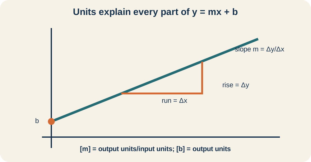
A linear model has the form $y=mx+b$. The coefficient $m$ is slope, meaning output change per unit input change. The constant $b$ is the output when input equals zero. If $x$ uses hours and $y$ uses dollars, slope uses dollars per hour. The intercept uses dollars.

Dimensional consistency requires $mx$ and $b$ to have the same units as $y$. Multiplying dollars per hour by hours produces dollars. Adding a bare number with no compatible units would be physically meaningless. Units therefore constrain which algebraic terms may be combined. They also clarify what a solved variable represents.

Suppose a service costs $C(t)=(18\,\frac{\mathrm{USD}}{\mathrm{h}})t+25\,\mathrm{USD}$. To find when the cost is $97\,\mathrm{USD}$, solve $(18\,\frac{\mathrm{USD}}{\mathrm{h}})t+25\,\mathrm{USD}=97\,\mathrm{USD}$. Subtraction gives $(18\,\frac{\mathrm{USD}}{\mathrm{h}})t=72\,\mathrm{USD}$. Division gives $t=4\,\mathrm{h}$, with currency units canceling properly. Substitution confirms that four hours produces the stated cost.

Translate verbal models before solving

Begin by defining the unknown with its units. Translate each phrase into a quantity rather than searching for isolated keywords. State assumptions about fixed rates, starting values, and feasible domains. Write the equation only after both sides represent the same kind of quantity. This sequence makes the equals sign a modeling claim.

Suppose a tank initially contains $12$ liters and fills at $3\,\frac{\mathrm{L}}{\mathrm{min}}$. Its volume after $t$ minutes is $V(t)=12\,\mathrm{L}+(3\,\frac{\mathrm{L}}{\mathrm{min}})t$. To find when it reaches $45$ liters, set the model equal to $45\,\mathrm{L}$. Solving gives $t=11\,\mathrm{min}$. The result assumes the rate stays constant and the tank has adequate capacity.

Reasonableness checks belong to the model. Time should not be negative in this context. Substitution should reproduce the target volume with matching units. A larger target should require a later time when the rate is positive. These checks can expose an incorrect sign or an implausible assumption.

Preserve inequalities between algebra and context

Not every modeled input is feasible even when the algebra yields a real number. Lengths may need to be positive, counts may need to be whole numbers, and times may be restricted to an operating interval. Record those constraints before solving. Compare each candidate with them afterward. A mathematically valid equation solution can still be inadmissible for the application.

Consider a rental plan modeled only for $0\le t\le24$ hours. Solving its cost equation might produce $t=30$ hours. That result satisfies an extrapolated formula but lies outside the stated model domain. The proper conclusion is that the target cost is not reached within the modeled interval. Extending the formula requires a new assumption.

Domain restrictions also arise from original algebraic expressions. A canceled denominator factor does not restore an excluded input. A square root or logarithm imposes its own conditions in later equations. Verification in the original statement detects many violations. Writing restrictions first ensures they are not forgotten after simplification.

Diagnose errors through invariants

An invariant is a property preserved through the solution process. For equivalent equation steps, the invariant is the solution set. Applying unequal operations to the two sides usually breaks it. Dividing by an expression that might be zero can lose valid cases. Multiplying by a variable expression can introduce values excluded by the original domain.

Distribution and combining like terms create common local errors. In $3(2x-1)$, the factor three multiplies both terms, giving $6x-3$. Terms combine only when their variable parts match. The expressions $6x$ and $1$ are not like terms. Structural reading should precede arithmetic.

Use substitution, graphs, and units as independent checks. Substitution tests the candidate in the original equation. Graphs show whether the expected number of intersections is plausible. Units test whether modeled terms and answers are dimensionally compatible. Independent evidence is especially useful because repeating the same algebra often repeats the same mistake.

Practice explaining rather than moving symbols

Solve $4(2x+3)-5=3x+22$ while naming every property. Distribute, combine constants, subtract the same variable term, and then subtract the same constant. Divide only after identifying a nonzero numerical coefficient. Substitute the candidate into both original sides. Record their common value as verification.

Next, classify $a(x-2)=ax+5$ for different values of the parameter $a$. Expand before deciding whether a variable coefficient remains. Notice that subtraction of $ax$ removes the variable for every parameter value. The remaining statement determines whether any solution exists. Explain why changing $a$ cannot create a unique solution in this family.

Finally, construct a linear model from a starting quantity and a constant rate. Label every coefficient with units. Solve for the input that reaches a chosen output and check the feasible domain. Interpret slope, intercept, and solution in complete sentences. The related lessons on graphing and systems will extend the same equality structure to multiple variables.

Sources and further study

OpenStax Elementary Algebra 2e develops properties of equality and linear-equation procedures. Its exercises provide extensive practice with fractions, variables on both sides, and applications. Rework examples while narrating the reversible operation on each line. Compare your candidate with the original equation. This turns procedural fluency into justified reasoning.

OpenStax Intermediate Algebra 2e extends linear reasoning into parameters, formulas, and systems. Use its graphs to connect solution sets with intersections. Identify domain restrictions before clearing variable denominators. Track units in every applied problem. These habits scale beyond linear equations.

Further study should connect equivalence to logic and linear algebra. Row operations on systems preserve solution sets for the same reversible reasons. Functions turn equations into intersection questions. Dimensional analysis constrains valid physical models. A concept map joining these ideas reveals linear equations as foundational structure rather than a narrow collection of steps.