Graphs Turn Relationships into Geometry

A coordinate graph turns paired numerical values into positions. Horizontal location records one variable, vertical location records another, and geometry makes their relationship visible. For a linear relationship, slope measures a constant rate of change and intercepts mark reference states. Equations, tables, verbal descriptions, and graphs are different representations of the same underlying pattern. Learning to translate among them makes a graph an analytical tool rather than a decorative picture.

Build the coordinate plane from two number lines

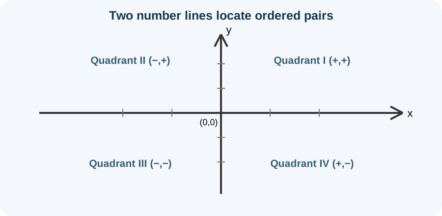
The Cartesian coordinate plane combines a horizontal number line and a vertical number line. Their intersection is the origin, written $(0,0)$. The horizontal axis is conventionally the $x$-axis. The vertical axis is conventionally the $y$-axis. Axis names may change when variables have meaningful names such as time $t$ or temperature $T$.

The axes divide the plane into four quadrants. Quadrant I contains points with positive $x$ and positive $y$. Moving counterclockwise, Quadrants II, III, and IV follow the sign patterns $(-,+)$, $(-,-)$, and $(+,-)$. Points on an axis belong to no quadrant. The signs of coordinates locate a point before exact distances are measured.

Axis ticks establish numerical scale. One square may represent one unit, ten units, or a fraction of a unit. Horizontal and vertical scales need not match. Labels and units therefore form part of the mathematical representation. An unlabeled plane cannot communicate what its positions mean.

Read an ordered pair in the correct order

An ordered pair $(x,y)$ names a point. The first coordinate gives horizontal displacement from the origin. The second gives vertical displacement. Parentheses group the coordinates into one location. Reversing their order generally produces a different point.

To plot $(3,-2)$, move three units right and two units down. To plot $(-2,3)$, move two units left and three units up. These points occupy different quadrants. Saying “along first, then up or down” reinforces the order. A quick projection to each axis checks the coordinates.

Coordinates require context. The point $(3,7)$ could mean three seconds and seven metres, three kilograms and seven dollars, or something else entirely. The horizontal coordinate usually represents an input or explanatory variable. The vertical coordinate usually represents an output or response. Axis titles convert abstract coordinates into a claim about paired quantities.

Translate a table into plotted points

A table records paired values in rows. If one row contains $x=2$ and $y=5$, the graph contains point $(2,5)$. Every row should be plotted using the same axis scales. Connecting points is justified only when intermediate inputs and outputs have meaning. Discrete categories should not automatically be joined by a continuous line.

Consider values satisfying $y=2x+1$. Inputs $0$, $1$, $2$, and $3$ produce outputs $1$, $3$, $5$, and $7$. The graph contains $(0,1)$, $(1,3)$, $(2,5)$, and $(3,7)$. Equal increases of one in $x$ produce equal increases of two in $y$. That constant change appears as collinearity.

A table can contain measurement noise, rounding, or outliers. Such points may not lie exactly on one line. A fitted line summarizes a trend rather than passing through every observation. Distinguish a mathematical relationship generated exactly from an equation from an empirical relationship estimated from data. The visual appearance alone does not establish exact linearity.

Define slope as a ratio of changes

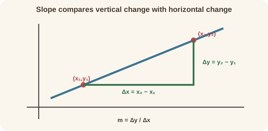
Between distinct points $(x_1,y_1)$ and $(x_2,y_2)$, slope is $m=\dfrac{y_2-y_1}{x_2-x_1}=\dfrac{\Delta y}{\Delta x}$. The Greek capital delta means change, computed as final minus initial. The horizontal fraction bar divides the complete vertical change by the complete horizontal change. The denominator must be nonzero. Slope measures output change per unit input change.

Using points $(2,5)$ and $(6,13)$ gives $m=\dfrac{13-5}{6-2}=\dfrac84=2$. The same result follows if point order is reversed because both numerator and denominator change sign. Mixing orders would produce an incorrect negative value. Writing each ordered pair in a vertical column helps preserve correspondence. The answer means two vertical units gained for every one horizontal unit.

Slope is constant along a nonvertical line. Any two distinct points on that line produce the same ratio. This constancy characterizes a linear relationship. A curved graph has changing secant slopes across different point pairs. Calculus later defines local slope through a limiting process.

Interpret slope signs and magnitudes

A positive slope means $y$ increases as $x$ increases. A negative slope means $y$ decreases as $x$ increases. Zero slope produces a horizontal line. A larger absolute value means more vertical change per horizontal unit. Sign describes direction, while magnitude describes rate steepness in numerical coordinates.

The phrase “steeper” depends on axis scale when judged visually. Numerical slope does not change if the graph is stretched on a screen, but the displayed angle does. Compare slopes using their calculated ratios rather than uncalibrated appearance. When units differ, even numerical magnitude comparisons may have limited meaning. A slope of three dollars per hour cannot be directly ranked against three metres per second as though they were one quantity.

A vertical line has undefined slope because $\Delta x=0$. Division by zero is not defined. Its equation has form $x=c$ for constant $c$. It cannot be written as $y=mx+b$ with finite $m$. It also fails the vertical line test for representing $y$ as a function of $x$.

Attach units to slope

Slope units are vertical-axis units divided by horizontal-axis units. If distance in metres is graphed against time in seconds, slope has units $\mathrm{m\,s^{-1}}$. It may represent velocity over an interval. If cost in dollars is graphed against mass in kilograms, slope has units dollars per kilogram. Units supply the rate’s physical meaning.

Suppose water volume rises from $10.0\,\mathrm L$ at $2.00\,\mathrm{min}$ to $22.0\,\mathrm L$ at $5.00\,\mathrm{min}$. The slope is $\dfrac{22.0\,\mathrm L-10.0\,\mathrm L}{5.00\,\mathrm{min}-2.00\,\mathrm{min}}=4.00\,\mathrm{L\,min^{-1}}$. This means volume increases by four litres per minute. The calculation retains units in numerator and denominator. A unitless answer would discard the application’s central interpretation.

Changing units changes the numerical slope. Four litres per minute equals $240\,\mathrm{L\,h^{-1}}$. The physical rate is unchanged even though the number differs. Therefore report both value and unit. Converting axes requires converting slope consistently.

Interpret intercepts as reference states

The $y$-intercept occurs where $x=0$. In equation $y=mx+b$, it is point $(0,b)$. The constant $b$ is the output associated with zero input. It may represent an initial amount, fixed charge, baseline reading, or mathematical extrapolation. Its contextual meaning depends on whether zero lies in the meaningful domain.

The $x$-intercept occurs where $y=0$. Set the output equal to zero and solve for $x$. For $y=-3x+7$, the intercept is $x=7/3$. Thus the point is $(7/3,0)$. It can represent a break-even input, depletion time, or crossing of a reference level.

An intercept can exist algebraically without being physically relevant. A temperature model fitted only from ten to twenty minutes may have a computed value at time zero outside the observed interval. A negative mass intercept may violate a domain restriction. Graphs should distinguish interpolation within supported inputs from extrapolation beyond them. Meaning comes from both equation and domain.

Use slope-intercept form

Slope-intercept form is $y=mx+b$. The coefficient $m$ gives slope, and constant $b$ gives the vertical intercept. Starting at $(0,b)$, a slope ratio provides another point. Repeating the rise and run generates the line. This form is efficient when rate and baseline are central.

For $y=-3x+7$, begin at $(0,7)$. Interpreting $-3$ as $-3/1$, move one unit right and three units down. The next point is $(1,4)$. Repeating gives $(2,1)$. Substitution verifies every point.

Not every line is conveniently expressed in this form. A vertical line has no finite slope. Equations with awkward fractions may be clearer in standard form. The best representation depends on the feature being studied. Converting forms should serve interpretation rather than become a ritual.

Use point-slope form

Point-slope form is $y-y_1=m(x-x_1)$. It describes the line with slope $m$ through known point $(x_1,y_1)$. The differences compare any point $(x,y)$ on the line with the fixed known point. Their ratio equals the slope. This form directly encodes the definition of constant rate.

For slope $-3$ through $(1,4)$, write $y-4=-3(x-1)$. Expanding gives $y-4=-3x+3$. Adding four gives $y=-3x+7$. Both forms describe the same line. Substituting $(1,4)$ into either equation confirms the point.

Point-slope form is useful when no intercept is given. It also reduces premature arithmetic. A common error is mismatching signs inside parentheses. The point $(1,4)$ produces $x-1$ and $y-4$, while a negative coordinate would produce addition after subtraction. Reading each difference as “variable minus coordinate” preserves the pattern.

Use standard form and intercepts

Standard form is often written $Ax+By=C$. Coefficients are commonly chosen as integers with a sign convention, though equivalent scalar multiples describe the same line. The variables appear symmetrically. This form makes intercepts easy to calculate. It also appears naturally in systems of equations.

Set $y=0$ to find the $x$-intercept $x=C/A$ when $A\neq0$. Set $x=0$ to find the $y$-intercept $y=C/B$ when $B\neq0$. For $2x+3y=12$, the intercepts are $(6,0)$ and $(0,4)$. Drawing the line through them gives a quick graph. Substitution checks both points.

Solving standard form for $y$ gives $y=-\dfrac ABx+\dfrac CB$ when $B\neq0$. Thus slope is $-A/B$. A missing $y$ term means a vertical line. A missing $x$ term means a horizontal line. Form conversion reveals these special cases.

Construct a line from two points

Two distinct points determine one line. First calculate their slope. Then substitute either point into point-slope form. Convert to another form only if useful. Finally, verify the second point.

Through $(2,5)$ and $(6,13)$, slope is two. Using the first point gives $y-5=2(x-2)$. Expansion produces $y=2x+1$. Substitution of $x=6$ gives $y=13$. This check confirms the line includes both points.

If the two points have equal $x$ coordinates, the line is vertical. For $(3,2)$ and $(3,8)$, its equation is $x=3$. Attempting the slope formula produces zero denominator. Recognizing the special case prevents forced use of slope-intercept form. The points still determine one valid line.

Move among equation, graph, table, and words

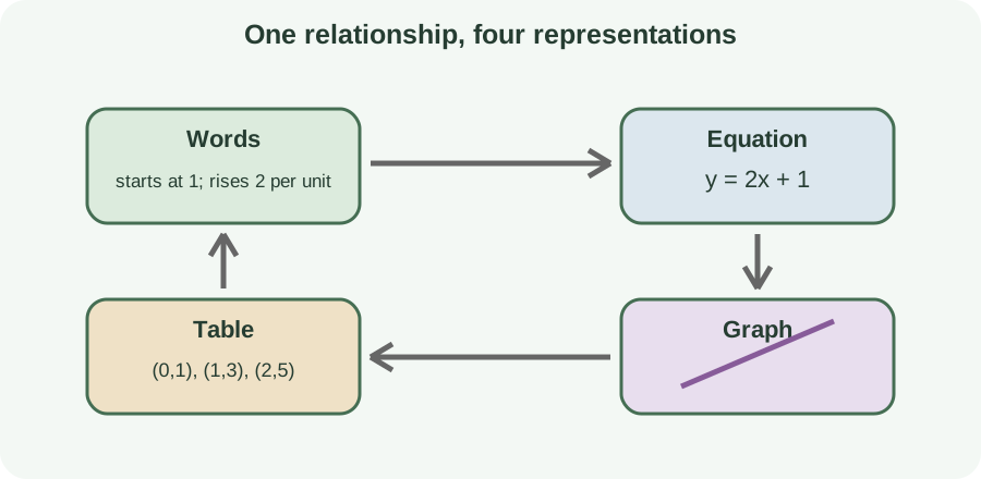
A complete understanding survives representation changes. Equation $y=2x+1$ states an output begins at one and increases two per input unit. A table shows repeated increments. A graph shows a line through $(0,1)$ with positive slope. Each representation highlights a different aspect.

From a graph, read two reliable points rather than estimating the visual angle. Compute slope and identify an intercept. Use those values to form an equation. From an equation, generate a small table using strategically chosen inputs. From words, identify rate and baseline before assigning symbols.

Translation also exposes ambiguity. “Starts at five and grows by three” needs units and an independent variable. “Three per hour” identifies a rate but not an initial value. “Passes through a point” does not establish a slope. Ask what information is present and what remains unknown.

Read intersections as simultaneous solutions

An intersection belongs to both graphs. Its coordinates satisfy both equations simultaneously. Therefore graphing can solve a system of equations. One intersection means one solution. Parallel distinct lines have none, while coincident lines have infinitely many.

Consider $y=2x+1$ and $y=-x+7$. At an intersection, their right sides are equal. Solving $2x+1=-x+7$ gives $x=2$ and $y=5$. The graph intersection is $(2,5)$. Substituting into both equations verifies the solution.

Graphical solutions may be approximate when the intersection falls between grid marks. Algebra can refine the coordinates. A graph still reveals whether a solution is plausible and unique. Using visual and symbolic methods together provides stronger evidence. Disagreement usually signals plotting, scaling, or algebra error.

Understand interpolation and extrapolation

Interpolation estimates an output between known or supported inputs. For a genuinely linear relationship, the line supplies exact intermediate values. For empirical data, interpolation assumes the trend remains adequate between observations. The estimate should include appropriate uncertainty. A graph makes the supported interval visible.

Extrapolation extends beyond observed or justified inputs. A straight line continues forever mathematically, but a real mechanism may change. A tank cannot fill indefinitely if it has finite capacity. A cost may change after a quantity discount. Long-range extrapolation requires stronger assumptions than interpolation.

Distinguish the function’s mathematical domain from the model’s practical domain. An equation may accept every real number while negative time or enormous input lacks meaning. Mark the intended interval on a graph. Interpret intercepts only when they belong to that interval. Responsible graphing communicates limitations as well as trends.

Detect misleading axis choices

Changing aspect ratio changes displayed steepness. A narrow graph can make modest changes look dramatic. A wide graph can flatten important variation. Numerical slope remains defined by axis values. Read tick labels before interpreting visual angle.

Truncating an axis can exaggerate differences. A bar or line varying from $98$ to $102$ looks extreme if the vertical axis begins at $97$. Truncation is not automatically dishonest, but it must be visible and suited to the question. Including a break or explicit minimum helps readers judge magnitude. Context determines whether zero is a necessary baseline.

Unequal intervals also mislead when drawn at equal spacing. Time points $1$, $2$, and $10$ must not occupy consecutive equal gaps on a numerical axis. Categorical axes follow different rules from quantitative axes. Grid spacing should match numerical distance. A technically correct equation can be visually misrepresented by an incorrect scale.

Diagnose common graphing errors

One error is reversing coordinates. Another is calculating rise and run with inconsistent point order. A third is ignoring units. A fourth is drawing through discrete categories as though intermediate values existed. Each error changes the claim the graph makes.

Students may also confuse $b$ with the $x$-intercept. In $y=mx+b$, $b$ is the output at $x=0$. Setting $y=0$ finds the other intercept. A negative slope does not imply a negative intercept. Rate and baseline are independent features.

Software does not eliminate these risks. It may choose an unhelpful window, connect points automatically, or hide labels. Enter parentheses carefully when fractions appear. Inspect the plotted domain and scale. Use algebraic checkpoints to validate the display.

Practice a complete linear interpretation

A line has slope $-3$ and passes through $(1,4)$. Point-slope form is $y-4=-3(x-1)$. Slope-intercept form is $y=-3x+7$. The vertical intercept is $(0,7)$. Setting $y=0$ gives horizontal intercept $(7/3,0)$.

Now attach a context. Suppose $x$ is elapsed time in hours and $y$ is water volume in litres. Slope $-3\,\mathrm{L\,h^{-1}}$ means volume decreases by three litres per hour. Intercept $7\,\mathrm L$ means the model predicts seven litres at time zero. The practical domain ends when volume reaches zero at $7/3\,\mathrm h$.

Finally, test the representation. Build a table at $x=0$, $1$, $2$, and $7/3$. Plot the points with labeled units. Confirm equal input increments produce equal output changes. Explain why extending beyond the zero-volume time would be mathematically possible but physically inappropriate.

Connect graphing to later mathematics

Linear graphs establish the language of rate and initial value. Functions generalize input-output relationships beyond straight lines. Systems use intersections to represent simultaneous constraints. Statistics uses fitted lines to summarize noisy data. Calculus transforms average slope into instantaneous derivative.

Coordinate geometry also supports distance, circles, and transformations. A slope condition can express parallel or perpendicular lines. Inequalities shade whole regions rather than single boundaries. Graphs of nonlinear functions retain axes, scale, intercept, domain, and representation checks. The foundational habits remain useful even when shapes become complex.

You are ready to continue when you can plot ordered pairs, calculate and interpret slope with units, and identify both intercepts. You should move among common line forms and distinguish visual steepness from numerical rate. You should read intersections as shared solutions and separate interpolation from extrapolation. These skills make graphs precise mathematical arguments. Later topics can then build on geometry that already carries quantitative meaning.