Electric Potential

Electric fields describe force per charge at every point in space. Electric potential describes potential energy per charge at those points. The field is a vector, while potential is a scalar. Both represent the same electrostatic interaction from different perspectives. Choosing between them can turn a difficult vector problem into simpler energy accounting.

Voltage is not a substance stored inside a wire. It is a difference in electric potential between two locations. A battery establishes a potential difference by using chemical processes to separate charge. A charged particle responds according to its own charge and the potential change. Keeping potential, potential energy, and charge distinct prevents many sign errors.

This lesson starts from energy-per-charge meaning before introducing formulas. It then develops reference levels, work, uniform fields, point-charge superposition, equipotential maps, conductors, and measurement. Every example identifies units and signs. Diagrams show how field arrows connect to potential contours. The goal is to reason about voltage rather than treat it as a calculator label.

Learning goals and an opening analogy

You should distinguish electric potential $V$ from electric potential energy $U$. You should calculate potential differences and energy changes. You should connect electric field to spatial potential change. You should add potentials from multiple point charges. You should interpret equipotentials and voltmeter readings.

Gravitational height provides a useful but limited analogy. Near Earth, greater height corresponds to greater gravitational potential energy per unit mass. Electric potential similarly describes electric potential energy per unit charge. The analogy helps with energy accounting. Electric charge can be positive or negative, which makes the electrical case richer.

Predict what happens to a positive test charge released in an electric field. Its electric potential energy decreases as the field does positive work. Because its charge is positive, it also moves toward lower electric potential. A negative charge can lower its energy by moving toward higher potential. The sign of the moving charge connects potential change to energy change.

Potential is energy per charge

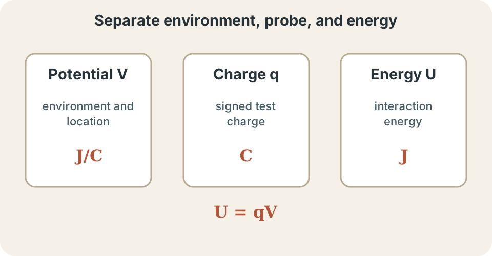
Electric potential at a point is defined by $V=\frac{U}{q}$ for the potential energy $U$ associated with a test charge $q$. The horizontal fraction means energy is divided by charge. Potential belongs to the source configuration and location, not to the chosen test charge. A sufficiently small test charge is imagined so it does not disturb the sources. The definition isolates the environment from the probe.

The SI unit is the volt, with $1\,\mathrm V=1\,\mathrm{\frac{J}{C}}$. One volt means one joule of potential energy per coulomb of positive charge. Multiplying potential by charge returns energy. Thus $(1\,\mathrm C)(1\,\mathrm{\frac{J}{C}})=1\,\mathrm J$. Unit cancellation mirrors the physical relationship $U=qV$.

Potential is a scalar even though electric field is a vector. Scalar values add algebraically without resolving spatial components. Their signs still matter. A negative potential is not inherently “bad” or impossible. It is measured relative to a selected zero and reflects source-charge signs.

Potential difference is voltage

Potential difference between final and initial points is $\Delta V=V_f-V_i$. The capital delta means final minus initial. Everyday language often calls this voltage. Voltage must therefore be specified between two nodes or locations. A single absolute reading requires an understood reference.

Potential-energy change is $\Delta U=q\Delta V$. Positive charge has energy change with the same sign as $\Delta V$. Negative charge reverses the sign. A neutral object has no point-charge electrostatic energy from this expression. Always insert the signed charge rather than only its magnitude.

If a $+2.00\,\mathrm{\mu C}$ charge moves through $\Delta V=-30.0\,\mathrm V$, then $\Delta U=(2.00\times10^{-6}\,\mathrm C)(-30.0\,\mathrm{\frac{J}{C}})=-6.00\times10^{-5}\,\mathrm J$. The negative result means electric potential energy decreases. The field can convert that decrease into kinetic energy if other transfers are absent. Units reduce explicitly from coulomb-volts to joules. The signed result is an energy change rather than an absolute energy.

Work and potential change

Conservative electrostatic work satisfies $W_{\mathrm{field}}=-\Delta U$. The negative sign means field work is positive when potential energy decreases. Combining this with $\Delta U=q\Delta V$ gives $W_{\mathrm{field}}=-q\Delta V$. External work in a slow controlled move is often $W_{\mathrm{ext}}=+\Delta U$. State which agent performs the work.

Suppose the previous positive charge moves through $-30.0\,\mathrm V$. Its energy change was $-6.00\times10^{-5}\,\mathrm J$. The electric field does $+6.00\times10^{-5}\,\mathrm J$ of work. If it starts from rest and only electric interaction matters, kinetic energy increases by that amount. The total mechanical-energy ledger balances.

Moving a negative charge toward higher potential can also lower potential energy. Let $q=-1.00\,\mathrm{\mu C}$ and $\Delta V=+20.0\,\mathrm V$. Then $\Delta U=(-1.00\times10^{-6})(20.0)=-2.00\times10^{-5}\,\mathrm J$. The field performs positive work. Potential direction alone does not determine energy direction without the charge sign.

Reference choices and gauge freedom

Potential energy requires a chosen zero. Adding the same constant to every potential does not change any potential difference. Electric fields and observable work remain unchanged. This freedom is sometimes called gauge freedom in elementary electrostatics. Only consistent differences enter ordinary predictions.

For isolated point charges, potential is conventionally set to zero infinitely far away. That choice makes $V=\frac{kq}{r}$ convenient. For a nearly uniform field between plates, one plate or a circuit ground may be chosen as zero. Neither reference is universally privileged. State it when absolute potential values matter.

A negative potential relative to infinity means a positive test charge would have negative potential energy at that point. It does not mean energy itself is universally below nothing. Reference shifts can change all potential values. Energy differences and work remain invariant. Physical interpretation should emphasize those invariant quantities.

Electric field and potential are linked

The potential difference generated by an electrostatic field is $\Delta V=-\int_i^f\mathbf E\boldsymbol\cdot d\mathbf l$. The integral adds the field component along each tiny displacement $d\mathbf l$. The centered dot denotes a dot product. The negative sign says potential decreases most rapidly in the field direction. Path independence follows for electrostatic fields.

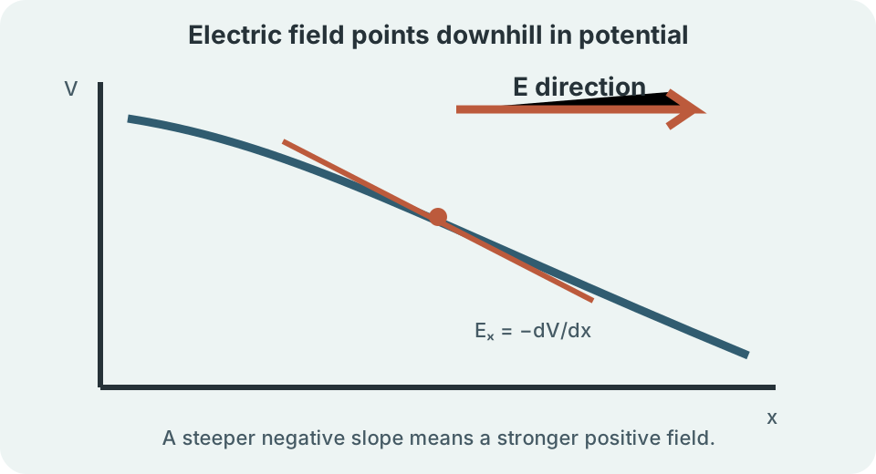
In one dimension, $E_x=-\frac{dV}{dx}$. Electric field is the negative spatial derivative of potential. A steep potential graph corresponds to a strong field magnitude. A flat region corresponds to zero field along that direction. Field depends on spatial change, not simply potential height.

In three dimensions, $\mathbf E=-\boldsymbol\nabla V$. The symbol $\boldsymbol\nabla$, called del, collects spatial partial derivatives. Its action on scalar $V$ produces the gradient vector. The negative gradient points downhill in potential. This relationship reconstructs a vector field from a scalar map.

Uniform fields

For a constant electric field parallel to displacement, the integral becomes $\Delta V=-E\Delta x$. This formula assumes the $x$ axis points along the field. Moving in the field direction gives positive $\Delta x$ and negative $\Delta V$. Moving against the field raises potential. Perpendicular displacement produces no potential change.

Between ideal large parallel plates, the central field is approximately uniform. If plate separation is $d$ and potential difference magnitude is $\Delta V$, then field magnitude is $E=\frac{|\Delta V|}{d}$. Units are $\mathrm{\frac{V}{m}}$. Because $1\,\mathrm{\frac{V}{m}}=1\,\mathrm{\frac{N}{C}}$, the energy and force descriptions agree. Edge fringing limits the approximation near plate boundaries.

A $12.0\,\mathrm V$ difference across $4.00\,\mathrm{mm}=4.00\times10^{-3}\,\mathrm m$ gives $E=\frac{12.0\,\mathrm V}{4.00\times10^{-3}\,\mathrm m}=3.00\times10^3\,\mathrm{\frac{V}{m}}$. The field points from higher to lower potential. A positive charge feels force with the field. A negative charge feels force opposite it. The numerical result applies to the approximately uniform central region.

Potential of a point charge

With zero potential at infinity, a point charge $Q$ produces $V(r)=\frac{kQ}{r}$. Here $r$ is positive distance from the source, and $k=8.99\times10^9\,\mathrm{\frac{N\,m^2}{C^2}}$. The source charge $Q$ retains its sign. Positive sources create positive potential relative to infinity. Negative sources create negative potential.

Units reduce correctly because $\mathrm{\frac{N\,m^2}{C^2}}\frac{C}{m}=\mathrm{\frac{N\,m}{C}}=\mathrm{\frac{J}{C}}=\mathrm V$. Potential magnitude decreases as distance increases. It varies as the reciprocal of $r$, not the reciprocal square. Electric field magnitude instead varies as $\frac{1}{r^2}$. Confusing these laws mixes energy-per-charge with force-per-charge.

At $r=0.200\,\mathrm m$ from $Q=+3.00\,\mathrm{nC}$, potential is $V=\frac{(8.99\times10^9)(3.00\times10^{-9})}{0.200}\,\mathrm V=135\,\mathrm V$. A $+1.00\,\mathrm{\mu C}$ test charge there has $U=qV=1.35\times10^{-4}\,\mathrm J$. The source determines $V$. The test charge determines how that potential becomes energy. Both quantities use zero potential at infinity.

Superposition of several charges

Potentials from point charges add as scalars. At a field point, $V=\sum_i\frac{kQ_i}{r_i}$. Each $r_i$ is the positive distance from source $Q_i$ to the field point. Each source charge retains its algebraic sign. No vector components are needed.

Suppose $+2.00\,\mathrm{nC}$ and $-2.00\,\mathrm{nC}$ are equally distant from a midpoint. Their potentials cancel at that point. Their electric fields generally do not cancel there because field directions must be considered. Zero potential does not imply zero electric field. Scalar cancellation and vector cancellation are different tests.

For multiple sources, draw the geometry and list each $Q_i$ and $r_i$. Compute signed terms before summing. A nearby small charge can contribute more potential magnitude than a distant larger charge. Check units and reference choice. Then multiply by a test charge only if potential energy is requested.

Potential energy of charge systems

Two point charges have mutual potential energy $U=\frac{kq_1q_2}{r_{12}}$ when zero is at infinite separation. The product $q_1q_2$ sets the sign. Like charges give positive energy. Opposite charges give negative energy. Separation $r_{12}$ is always positive.

Positive energy for like charges means external work is required to assemble them from infinity slowly. Negative energy for opposite charges means the field releases energy during assembly. Separating an attractive pair back to infinity requires positive external work. These interpretations depend on the chosen zero. Work differences remain physical.

For many charges, sum each distinct pair once: $U=\sum_{i<j}\frac{kq_iq_j}{r_{ij}}$. The condition $i<j$ prevents double counting. Alternatively, assemble charges sequentially and use existing potential at each insertion. Do not include a charge’s self-potential in the elementary point-charge model. Pair accounting and assembly accounting must agree.

Equipotential surfaces

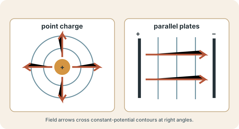
An equipotential surface contains points with the same potential. Moving a test charge along it gives $\Delta V=0$. Electrostatic field work is therefore zero along that displacement. The field has no tangential component on an equipotential. It crosses equipotential surfaces perpendicularly.

Closer equipotential spacing indicates a larger potential gradient and stronger field. Wide spacing indicates weaker field. The numerical contour interval must be known before comparing maps. Equal drawn spacing with different voltage intervals does not represent equal fields. Map scale also matters.

Around an isolated point charge, equipotentials are concentric spheres. In a two-dimensional drawing, they appear as circles. Between ideal parallel plates, equipotentials are planes parallel to the plates. Complex source arrangements produce distorted contours. Field arrows always point toward decreasing potential.

Conductors in electrostatic equilibrium

Inside an ideal conductor at electrostatic equilibrium, electric field is zero. Otherwise mobile charges would continue moving. Because $\mathbf E=-\boldsymbol\nabla V$, zero internal field means potential is constant throughout the conductor. Its surface is also an equipotential. This conclusion applies after equilibrium is established.

Excess charge resides on the surface in the ideal electrostatic model. The field immediately outside is perpendicular to the surface. A tangential component would drive surface charge motion. Charge density becomes greater near sharp curvature. Strong local fields can promote discharge in surrounding material.

A conductor can have nonzero potential while its internal field is zero. Constant potential is not the same as zero potential. Grounding can set a conductor’s potential relative to Earth by allowing charge exchange. The amount of charge needed depends on geometry and nearby objects. Potential and field answer different questions.

Voltage measurement and circuits

A voltmeter measures potential difference between two probes. The displayed sign depends on probe ordering. If the red probe is at higher potential than the reference probe, a conventional meter reads positive. Reversing probes reverses the sign. The same two physical nodes remain involved.

An ideal voltmeter has infinite resistance and draws no current. A real meter has high finite input resistance. Connecting it in parallel can alter a high-resistance circuit. This loading changes the voltage being measured. Measurement devices belong in a complete circuit model when precision matters.

Circuit ground is a chosen reference node, not necessarily literal Earth. Assigning it $0\,\mathrm V$ simplifies node potentials. A $5.0\,\mathrm V$ node is five volts above that reference. Voltage across a component is the difference between its endpoint node potentials. Circuit analysis therefore applies the same potential-difference concept.

Electron-volts and energy scale

The electron-volt is a unit of energy, not potential. One electron-volt is the energy magnitude gained by elementary charge moving through one volt. Numerically, $1\,\mathrm{eV}=1.602\times10^{-19}\,\mathrm J$. The abbreviation eV should not be confused with a product left unevaluated. It is a named energy unit.

An electron moving through a potential rise of $100\,\mathrm V$ has potential-energy change $\Delta U=q\Delta V=(-e)(100\,\mathrm V)=-100\,\mathrm{eV}$. If only the field acts, its kinetic energy can increase by $100\,\mathrm{eV}$. The negative electron charge reverses the energy sign. Energy conservation supplies the kinetic interpretation. The potential rise and energy decrease are therefore compatible.

Electron-volts are convenient for atomic and particle scales. Joules remain the SI energy unit for dimensional calculations. Convert only when needed. Always distinguish a potential difference in volts from an energy in electron-volts. The similar names encode a precise charge-times-voltage relationship.

Common misconceptions and repairs

One misconception says electric potential and potential energy are the same. Potential belongs to a location and source configuration. Potential energy also depends on the placed charge through $U=qV$. Two test charges at one location share $V$ but can have different $U$. Attach units to expose the difference.

Another misconception says charges always move toward lower potential. Positive charges tend that way when released. Negative charges tend toward higher potential while still lowering their potential energy. Force direction follows $\mathbf F=q\mathbf E$. Charge sign must remain explicit.

A third misconception says zero potential means zero field. Equal positive and negative scalar contributions can cancel potential while vector field remains. Conversely, a region can have constant nonzero potential and zero field. Potential height and potential slope are distinct. Check the gradient rather than the value alone.

A reliable problem-solving routine

Define source charges, test charge, initial point, final point, and potential reference. Decide whether the requested quantity is $V$, $\Delta V$, $U$, $\Delta U$, work, or field. Predict signs before calculating. Draw distances from every source to the field point. Keep source and test charges conceptually separate.

Use scalar superposition for potential. Use $\Delta U=q\Delta V$ only after finding potential change. Use $W_{\mathrm{field}}=-\Delta U$ to identify field work. Use $\mathbf E=-\boldsymbol\nabla V$ or its one-dimensional form for spatial change. Carry volts, coulombs, joules, and metres explicitly.

Check whether the result depends appropriately on charge sign and distance. Confirm that point-charge potential follows $\frac{1}{r}$ rather than $\frac{1}{r^2}$. Verify that field points downhill in potential. State reference and idealizations. Finish by translating the sign into an energy or direction statement.

Practice and connection forward

A $+4.00\,\mathrm{\mu C}$ charge moves through $\Delta V=+25.0\,\mathrm V$. Its energy change is $\Delta U=(4.00\times10^{-6}\,\mathrm C)(25.0\,\mathrm{\frac{J}{C}})=1.00\times10^{-4}\,\mathrm J$. The field does $-1.00\times10^{-4}\,\mathrm J$ of work. Positive energy change means an external agent would supply energy in a slow move. All signs follow the chosen initial and final points.

A $-3.00\,\mathrm{nC}$ point charge creates potential at $0.150\,\mathrm m$. Using infinity as zero gives $V=\frac{(8.99\times10^9)(-3.00\times10^{-9})}{0.150}\,\mathrm V=-180\,\mathrm V$. The negative sign comes from the source charge. A positive test charge there has negative potential energy. A negative test charge there has positive potential energy.

Without looking back, explain volts as joules per coulomb and distinguish $V$ from $U$. Explain why field arrows cross equipotentials perpendicularly. Give an example where $V=0$ but $\mathbf E\ne0$. Circuit lessons will use potential differences to drive current. Capacitance will connect stored charge, voltage, field, and energy.