Electric Field

Electric interactions can occur even when charged objects do not touch. The field model explains this apparent action at a distance by assigning an electric influence to every point in space. A source charge establishes the field, and another charge responds to the field where it is located. Separating those two roles is the central idea of this lesson. By the end, you will be able to move deliberately among words, vectors, diagrams, and calculations instead of treating the electric-field formula as an isolated rule.

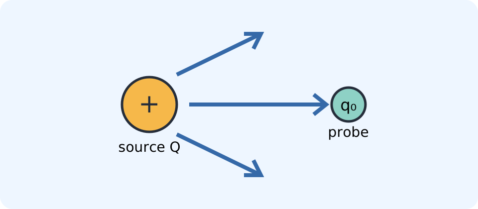
Begin with source, field, and response

A charged source changes the physical conditions in the space around it. We describe those conditions with the electric-field vector $\mathbf{E}$, where bold type indicates that the quantity has both magnitude and direction. The field exists whether or not another charged particle is placed nearby. A test charge is therefore a probe, not the cause of the field being measured. This distinction prevents the common mistake of including the test charge in a formula for the source field.

Imagine first placing a small positive charge at several locations around a fixed source. At each location, measure the electric force $\mathbf{F}$ on the probe and divide by the probe charge $q_0$. If the probe is sufficiently small that it does not rearrange the sources, the ratio is a property of the location. The operational definition is $\mathbf{E}=\dfrac{\mathbf{F}}{q_0}$. The subscript zero identifies the charge as a test charge rather than one of the sources.

This definition says that electric field is force per unit positive charge. Its SI unit is the newton per coulomb, written $\mathrm{\dfrac{N}{C}}$, and dimensional analysis follows directly from force divided by charge. A field of $200\,\mathrm{\dfrac{N}{C}}$ means that each coulomb of positive charge would experience $200\,\mathrm{N}$ of force at that point. A one-coulomb test charge is usually impractical because it is extraordinarily large on laboratory scales. The phrase “per coulomb” describes a ratio, not a required experimental probe.

Predict the response of a charge

Once a source field is known, the force on an inserted charge follows from $\mathbf{F}=q\mathbf{E}$. Here $q$ is the responding charge, $\mathbf{E}$ is the preexisting field at its position, and $\mathbf{F}$ is the electric force on it. Multiplying $\mathrm{C}$ by $\mathrm{\dfrac{N}{C}}$ leaves $\mathrm{N}$, so the units confirm the relation. The equation also keeps the source and response stages separate. Calculate the field from its sources first, then use that field to calculate the force on the chosen object.

The sign of $q$ controls the force direction. A positive charge experiences force in the same direction as $\mathbf{E}$, because multiplying a vector by a positive scalar preserves direction. A negative charge experiences force opposite $\mathbf{E}$, because multiplying by a negative scalar reverses direction. The field itself does not reverse merely because a negative probe is used. Field direction is defined by the force that a hypothetical positive test charge would experience.

Consider an electron in a uniform eastward field of $2.00\times10^4\,\mathrm{\dfrac{N}{C}}$. Its charge is $q=-1.602\times10^{-19}\,\mathrm{C}$, so the magnitude of its force is $|\mathbf{F}|=|q|E=(1.602\times10^{-19}\,\mathrm{C})(2.00\times10^4\,\mathrm{\dfrac{N}{C}})=3.20\times10^{-15}\,\mathrm{N}$. The negative sign does not make the magnitude negative; it tells us that the force points west, opposite the field. Stating both magnitude and direction completes a vector answer. Notice that every numerical value carries a unit and that the coulomb units cancel visibly.

Derive the field of a point charge

Coulomb’s law gives the force between an isolated source charge $Q$ and a test charge $q_0$. In vector form, the force on the test charge is $\mathbf{F}=k_e\dfrac{Qq_0}{r^2}\hat{\mathbf{r}}$. The constant $k_e=8.988\times10^9\,\mathrm{\dfrac{N\,m^2}{C^2}}$, the distance $r$ runs from the source to the field point, and $\hat{\mathbf{r}}$ is a unit vector pointing radially outward from the source. A unit vector has magnitude one and communicates direction without changing the numerical magnitude. Dividing this force by $q_0$ produces the field independently of the probe.

The resulting expression is $\mathbf{E}=k_e\dfrac{Q}{r^2}\hat{\mathbf{r}}$. If $Q$ is positive, the coefficient is positive and the field points along $\hat{\mathbf{r}}$, outward from the source. If $Q$ is negative, the coefficient is negative and the field points opposite $\hat{\mathbf{r}}$, inward toward the source. The inverse-square factor means that doubling $r$ reduces the magnitude to one fourth. Tripling $r$ reduces it to one ninth, so distance often matters more strongly than intuition first suggests.

Suppose $Q=+2.00\,\mathrm{\mu C}$ and the field point is $0.300\,\mathrm{m}$ to its right. Converting the prefix gives $Q=2.00\times10^{-6}\,\mathrm{C}$, and substitution gives $E=(8.988\times10^9\,\mathrm{\dfrac{N\,m^2}{C^2}})\dfrac{2.00\times10^{-6}\,\mathrm{C}}{(0.300\,\mathrm{m})^2}=2.00\times10^5\,\mathrm{\dfrac{N}{C}}$. The squared metres cancel, and one coulomb in the denominator remains, exactly as the field unit requires. Because the positive source lies to the left, the outward field at the chosen point is rightward. A complete result is therefore $2.00\times10^5\,\mathrm{\dfrac{N}{C}}$ to the right.

Add fields through superposition

Real configurations often contain more than one source charge. The principle of superposition says that each source contributes the field it would create alone, and the net field is the vector sum $\mathbf{E}_{\text{net}}=\sum_i\mathbf{E}_i$. The capital Greek sigma $\sum$ means “add the following quantity over all indexed sources.” The index $i$ labels each source, so $\mathbf{E}_i$ is the field contribution from source number $i$. Every contribution is evaluated at the same observation point even though the sources occupy different positions. Because fields are vectors, their directions must be resolved before their magnitudes are combined.

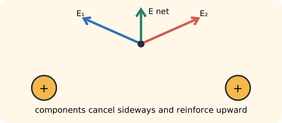
A reliable procedure begins with a sketch and a coordinate system. Mark the field point, draw the direction of every contribution there, and calculate each magnitude using its own source distance. Next resolve oblique vectors into components such as $E_x=E\cos\theta$ and $E_y=E\sin\theta$. Add signed components to obtain $E_{\text{net},x}$ and $E_{\text{net},y}$, then reconstruct the magnitude with $E_{\text{net}}=\sqrt{E_{\text{net},x}^2+E_{\text{net},y}^2}$. This method makes cancellation and reinforcement visible instead of leaving them to guesswork.

As a one-dimensional example, place $+3.00\,\mathrm{\mu C}$ at $x=0\,\mathrm{m}$ and $-3.00\,\mathrm{\mu C}$ at $x=0.400\,\mathrm{m}$. At the midpoint, each source is $0.200\,\mathrm{m}$ away and creates magnitude $E=(8.988\times10^9\,\mathrm{\dfrac{N\,m^2}{C^2}})\dfrac{3.00\times10^{-6}\,\mathrm{C}}{(0.200\,\mathrm{m})^2}=6.74\times10^5\,\mathrm{\dfrac{N}{C}}$. The positive charge’s field points away from it, to the right, while the negative charge’s field points toward it, also to the right. The contributions reinforce, giving $E_{\text{net}}=1.35\times10^6\,\mathrm{\dfrac{N}{C}}$ to the right. Equal source magnitudes do not guarantee cancellation because direction depends on both charge sign and observation point.

Read field-line diagrams critically

Field lines are a visual language for a vector field, not physical threads in space. At any ordinary point, the tangent to a field line gives the direction of $\mathbf{E}$. Closely spaced lines conventionally indicate a stronger field, while widely spaced lines indicate a weaker field. Lines begin on positive charge and end on negative charge or extend to infinity when an opposite charge is unavailable. The number of lines drawn is a representational choice, so only relative density within a consistently drawn diagram should be compared.

Field lines never cross. If two lines crossed, their tangents would assign two different field directions to the same point, contradicting the definition of a vector field. A moving positive particle may initially accelerate tangent to a line, but its full trajectory need not follow that line because velocity and inertia also matter. A negative particle initially accelerates opposite the line direction. Reading a field-line picture as a map of possible particle paths therefore confuses a spatial property with a time-dependent motion.

Symmetry provides a powerful check on these diagrams. An isolated point charge must have a radial pattern because no sideways direction is physically preferred. Equal like charges produce a perpendicular-bisector cancellation point at their midpoint, whereas equal opposite charges produce reinforcing fields between them. Far from a compact group of charges, the pattern may resemble that of the group’s net charge. Before calculating, use these qualitative facts to predict directions and approximate regions of strong or weak field.

Connect electric field to acceleration

The electric field determines force, but Newton’s second law determines motion. Combining $\mathbf{F}=q\mathbf{E}$ with $\mathbf{F}=m\mathbf{a}$ gives $\mathbf{a}=\dfrac{q}{m}\mathbf{E}$ for a particle of mass $m$. The ratio $\dfrac{q}{m}$ is the charge-to-mass ratio, and it controls how strongly a particle accelerates in a given field. Two particles with equal charge but different mass experience equal force yet different acceleration. This distinction is essential when comparing electrons, protons, ions, and macroscopic charged objects.

In a uniform field, a particle’s acceleration is constant if other forces can be neglected. The familiar constant-acceleration equations can then describe its motion, but the sign of $q$ must be included when determining acceleration direction. If the initial velocity is perpendicular to the field, the motion resembles projectile motion: uniform motion in one direction and accelerated motion in the other. If velocity is parallel or antiparallel to the field, the particle speeds up or slows down along a line. The field diagram alone does not specify the path because the initial velocity is additional information.

For an electron, $m_e=9.109\times10^{-31}\,\mathrm{kg}$ and $|q_e|=1.602\times10^{-19}\,\mathrm{C}$. In a field of $500\,\mathrm{\dfrac{N}{C}}$, its acceleration magnitude is $a=\dfrac{|q_e|E}{m_e}=\dfrac{(1.602\times10^{-19}\,\mathrm{C})(500\,\mathrm{\dfrac{N}{C}})}{9.109\times10^{-31}\,\mathrm{kg}}=8.79\times10^{13}\,\mathrm{\dfrac{m}{s^2}}$. The large value reflects the electron’s tiny mass rather than an unusually large force. Its acceleration points opposite the field because its charge is negative. This example also shows why units should remain attached throughout a calculation instead of being added only at the end.

Understand conductors in electrostatic equilibrium

A conductor contains charges that can move through the material. Electrostatic equilibrium means that the macroscopic charge distribution has stopped changing and no sustained electric current flows. If a nonzero electric field remained inside an ideal conductor, mobile charges would accelerate and the state would not be equilibrium. Therefore the electric field inside the conducting material is zero under electrostatic conditions. This statement is conditional and should not be carried uncritically into circuits with current or situations with changing electromagnetic fields.

Excess charge on an isolated conductor resides on its surface at equilibrium. The electric field immediately outside that surface is perpendicular to it, because a tangential component would drive surface charges sideways. Surface curvature affects charge concentration, with sharper regions often supporting greater surface-charge density. Greater density generally corresponds to a stronger nearby field. These results explain electrostatic shielding and the enhanced fields near pointed conductors.

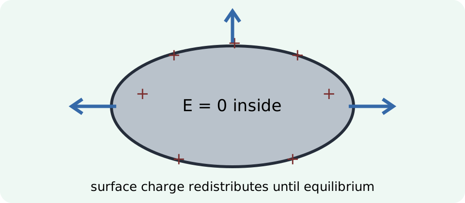
A hollow conductor can shield its cavity from external static electric fields when no charge is placed inside the cavity. This is the electrostatic basis of a Faraday cage, although practical enclosures have openings, finite conductivity, and frequency-dependent behavior. The shielding claim does not mean that every field everywhere near a conductor is zero. The exterior field can be strong, and a charge inside a cavity changes the induced surface-charge pattern. Always identify the region and physical conditions before applying the equilibrium rules.

Repair common misconceptions

One common error is to write $E=k_e\dfrac{Qq}{r^2}$, which is actually the magnitude of force rather than field. The source-field expression contains only the source charge $Q$. The responding charge $q$ enters later through $\mathbf{F}=q\mathbf{E}$. Keeping a two-column record labeled “source” and “response” can make this separation habitual. Unit checking catches the same error because the extra coulomb produces newtons instead of newtons per coulomb.

A second error is to add field magnitudes without considering direction. Equal contributions may reinforce, cancel, or combine at an angle, so a sketch must precede arithmetic. A third error is to assume that “negative field” means weak field. A negative component communicates direction relative to a chosen positive axis, whereas magnitude is nonnegative. The vector $\mathbf{E}=(-300\,\hat{\mathbf{x}}+400\,\hat{\mathbf{y}})\,\mathrm{\dfrac{N}{C}}$ has magnitude $500\,\mathrm{\dfrac{N}{C}}$, not $100\,\mathrm{\dfrac{N}{C}}$.

A final error is to treat field lines as literal objects or guaranteed trajectories. A field line encodes the direction of the field at many positions, while a trajectory records one object’s position over time. Particle motion depends on charge sign, mass, initial velocity, and all forces present. Asking “what information does this representation omit?” is an effective self-check. Good diagrams support reasoning, but they never replace the physical definitions beneath them.

Practice deliberately

First, find the field $0.250\,\mathrm{m}$ to the left of a $-4.00\,\mathrm{\mu C}$ point charge. Predict the direction before calculating, convert microcoulombs to coulombs, and retain the squared distance with its unit. The magnitude is $5.75\times10^5\,\mathrm{\dfrac{N}{C}}$. Because the field points toward a negative source, the direction is to the right. Explain why a negative test charge placed there would feel force to the left.

Second, a proton enters a uniform upward field of $1.20\times10^3\,\mathrm{\dfrac{N}{C}}$. Use $q_p=+1.602\times10^{-19}\,\mathrm{C}$ and $m_p=1.673\times10^{-27}\,\mathrm{kg}$ to find its force and acceleration. The force is $1.92\times10^{-16}\,\mathrm{N}$ upward, and the acceleration is $1.15\times10^{11}\,\mathrm{\dfrac{m}{s^2}}$ upward. The shared direction follows from the proton’s positive charge. Compare this acceleration with the electron example and attribute the difference quantitatively to charge-to-mass ratio.

Third, sketch two equal positive charges and identify the net-field direction at the exact midpoint, above the midpoint, and far to the right. At the midpoint the two equal and opposite contributions cancel. Above the midpoint, horizontal components cancel while vertical components reinforce upward. Far to the right, both fields point mainly rightward and reinforce. Describe these conclusions in words before attempting component calculations, because prediction is part of solution verification rather than an optional decoration.

Consolidate the model

The conceptual chain is source charge $\longrightarrow$ electric field $\longrightarrow$ force $\longrightarrow$ acceleration. Each arrow represents a different relationship and introduces different information. Coulomb’s law or superposition determines the field from sources, $\mathbf{F}=q\mathbf{E}$ determines a response force, and $\mathbf{a}=\dfrac{\mathbf{F}}{m}$ determines motion. Mixing these stages is responsible for many sign and variable errors. Writing the chain at the top of a solution gives every quantity a clear physical role.

Your reasoning should also move among multiple representations. Words establish cause and direction, sketches expose geometry, equations quantify the relationships, and units test whether the algebra remains physically meaningful. A correct numerical magnitude paired with a wrong direction is not a complete vector solution. A beautiful field-line drawing unsupported by source signs is not a complete explanation. Durable understanding appears when all four representations agree.

Electric potential will provide a complementary scalar description measured in joules per coulomb, or volts. Potential is often easier to add because scalars have no direction, but field remains necessary for predicting force. Later, the relation between potential and field will show that the electric field points in the direction of most rapid potential decrease. Keep the present source-field-response model intact as that new representation is introduced. It will serve as the organizing structure for electrostatics, circuits, and eventually electromagnetic theory.