Electric Charge and Coulomb’s Law

Electric charge is a conserved property of matter associated with electric interaction. Charges can attract or repel, unlike masses in ordinary Newtonian gravity, which attract in the foundational model. The two charge signs are called positive and negative. Like signs repel, and unlike signs attract. Coulomb’s law quantifies the force between stationary point charges.

Charge can move between objects without being created or destroyed in an isolated system. It occurs in discrete multiples of the elementary charge magnitude. In materials, mobile charges respond differently depending on electrical structure. Conductors allow charge redistribution over large distances, while insulators more strongly localize charge. Neutral objects can still experience electric forces through polarization.

This lesson builds Coulomb’s law as a vector relationship rather than a sign recipe. It develops direction, magnitude, units, superposition, symmetry, and equilibrium. Worked examples keep metres and coulombs explicit. Comparisons with gravity clarify the inverse-square form while preserving physical differences. The final workflow states when point-charge and electrostatic assumptions are justified.

Learning objectives and opening observations

After this lesson, you should distinguish charge sign, amount, and location. You should use conservation and quantization in transfer problems. You should calculate Coulomb-force magnitude with SI units. You should determine force direction geometrically and add multiple contributions as vectors. You should evaluate the point-charge approximation.

Rub a plastic object with another material and it may attract small neutral paper pieces. This does not prove the paper had opposite net charge initially. The charged object polarizes the paper, producing closer opposite-sign regions and farther like-sign regions. Because electric force depends strongly on distance, the nearer attraction can dominate. Neutrality does not imply absence of electric response.

Bring two similarly charged lightweight objects near one another and they repel. Oppositely charged objects attract. These observations define the empirical sign rule. The labels positive and negative are conventions. Their physical significance lies in how charges interact and move.

Charge is conserved

Charge conservation states that total electric charge of an isolated system remains constant. Charge can transfer between objects. Positive and negative particles can be separated or recombined. Pair-production processes preserve net charge even in advanced physics. A complete system boundary is essential.

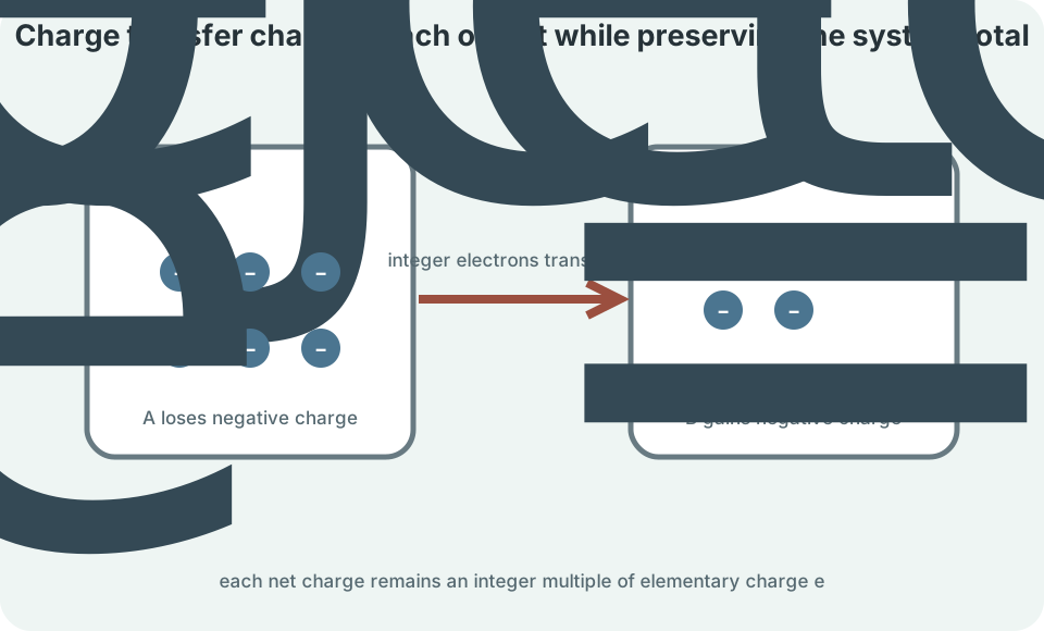
If an initially neutral object loses electrons, it becomes positively charged. The removed electrons carry negative charge to another object or environment. Protons generally remain bound in atomic nuclei during ordinary charging. Saying an object “gains positive charge” can hide the actual electron transfer. Track particles and system boundaries.

Suppose object A begins with charge $-3.0\,\mathrm{\mu C}$ and transfers $1.0\,\mathrm{\mu C}$ of negative charge to neutral object B. Object A becomes $-2.0\,\mathrm{\mu C}$, while B becomes $-1.0\,\mathrm{\mu C}$. Total remains $-3.0\,\mathrm{\mu C}$. Signs must accompany every amount. Conservation checks the bookkeeping.

Charge is quantized

Net charge occurs in integer multiples of elementary charge magnitude $e=1.602176634\times10^{-19}\,\mathrm C$. The unit $\mathrm C$ is coulombs. An electron has charge $-e$, and a proton has charge $+e$. If an object has net charge $q$, then $q=ne$ for integer $n$ in ordinary charge counting. The sign of $n$ indicates excess charge type.

A charge of $-4.80\times10^{-9}\,\mathrm C$ corresponds to electron-count difference $n=\frac{-4.80\times10^{-9}\,\mathrm C}{1.602\times10^{-19}\,\mathrm C}\approx-3.00\times10^{10}$. Coulomb units cancel in the ratio. The negative sign indicates excess electrons. The magnitude is about thirty billion particles. Rounding reflects the three significant figures in the measured charge.

Macroscopic charges involve enormous particle counts, so charge can appear continuous at everyday scales. Quantization remains fundamental. A calculated electron count should be an integer within measurement uncertainty. If it is far from an integer for a tiny controlled system, assumptions or data require review. Reported macroscopic charge uncertainty may hide individual increments.

Conductors and insulators redistribute charge differently

In a conductor, some charge carriers can move through the material over macroscopic distances. Metals contain mobile electrons. When excess charge is placed on an isolated conductor, it redistributes until electrostatic equilibrium is reached. The electric field inside the conducting material is then zero in the ideal static state. Excess charge resides on its surface.

In an insulator, charges are more tightly bound to local atoms or molecules. Deposited charge can remain localized for long periods. The material can still polarize as positive and negative regions shift slightly. “Insulator” does not mean electrically unaffected. It means long-range charge motion is strongly restricted under the conditions.

Grounding connects an object to a large charge reservoir such as Earth. Electrons can flow to or from the object depending on potential differences and nearby charges. Grounding does not always remove every local polarization effect. The sequence of contact and separation matters in induction. Draw each step in a charging process.

Polarization explains attraction of neutral matter

A charged rod near a neutral conductor causes mobile charge to redistribute. Opposite-sign charge accumulates closer to the rod, while like-sign charge shifts farther away. Net charge remains zero if no charge enters or leaves. The spatial separation forms an induced dipole. The closer attractive interaction can exceed the farther repulsive interaction.

An insulator can polarize through small shifts of bound charges or molecular orientation. The response may be weaker or slower than in a conductor. Neutral molecules with permanent dipoles can also rotate in an electric field. Thermal motion opposes perfect alignment. Material response depends on structure and temperature.

Polarization is evidence that net charge alone does not determine force. Distribution matters. A point-charge model compresses a small spherically symmetric distribution into one location. It cannot describe induced redistribution in an extended nearby object without additional modeling. Choose the model that matches scale and geometry.

Coulomb’s law gives point-charge force magnitude

For two stationary point charges separated by distance $r$, force magnitude is $F=k\frac{|q_1q_2|}{r^2}$. The symbols $q_1$ and $q_2$ are charges, $r$ is center-to-center separation, and $k$ is Coulomb’s constant. In vacuum, $k\approx8.99\times10^9\,\mathrm{\frac{N\,m^2}{C^2}}$. Absolute value keeps magnitude nonnegative. Charge signs determine direction separately.

The inverse square means doubling distance reduces force magnitude to one fourth. Tripling distance reduces it to one ninth. Doubling one charge doubles force. Doubling both charges multiplies force by four. Proportional reasoning provides quick checks before arithmetic.

The law assumes point charges or spherically symmetric charge distributions observed externally. The charges must be effectively stationary for electrostatics. The surrounding medium can modify interaction through permittivity. At atomic scales, quantum mechanics becomes essential. A formula is inseparable from its domain.

Coulomb force is a vector

The force on charge 2 due to charge 1 can be written $\mathbf F_{1\to2}=k\frac{q_1q_2}{r_{12}^2}\hat{\mathbf r}_{1\to2}$. The unit vector $\hat{\mathbf r}_{1\to2}$ points from charge 1 toward charge 2. The signed product determines whether the force follows or opposes that direction. Alternative vector conventions are possible. Define the unit vector before using signs.

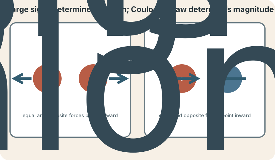
If $q_1q_2>0$, charges have the same sign and repel. Charge 2 is pushed away from charge 1, along $\hat{\mathbf r}_{1\to2}$. If $q_1q_2<0$, they attract. Charge 2 is pulled toward charge 1, opposite the unit vector. A sketch is safer than memorizing algebraic sign alone.

Newton’s third law gives $\mathbf F_{1\to2}=-\mathbf F_{2\to1}$. The forces have equal magnitude and opposite direction. They act on different objects and therefore do not cancel on one object’s free-body diagram. The pair conserves momentum for the closed interacting system. Label force subscripts carefully.

Worked two-charge example

Let $q_1=+2.00\,\mathrm{\mu C}$ and $q_2=-3.00\,\mathrm{\mu C}$ be separated by $r=0.500\,\mathrm m$. Convert microcoulombs using $1\,\mathrm{\mu C}=10^{-6}\,\mathrm C$. The force is attractive because the charge product is negative. Compute magnitude from absolute values. Keep the separation squared.

Substitution gives $F=\left(8.99\times10^9\,\mathrm{\frac{N\,m^2}{C^2}}\right)\frac{(2.00\times10^{-6}\,\mathrm C)(3.00\times10^{-6}\,\mathrm C)}{(0.500\,\mathrm m)^2}=0.216\,\mathrm N$. Coulomb squared cancels between constant and charges. Metre squared cancels between constant and separation. The result therefore has newtons. Three significant figures match the supplied values.

Each charge experiences force magnitude $0.216\,\mathrm N$ toward the other. Their accelerations need not match because their masses can differ. Force equality follows from interaction symmetry. Acceleration follows after dividing each force by its own mass. Do not infer identical motion from equal force magnitude.

Superposition adds force contributions

With several source charges, total force on a chosen target is the vector sum of individual pair forces. Write $\mathbf F_{\mathrm{net}}=\sum_i\mathbf F_{i\to\mathrm{target}}$. The index $i$ runs over source charges. Compute each contribution as if the others were present but did not alter the Coulomb-law calculation. Then add components.

Superposition follows linearity of the electric field and force for a fixed test charge. It does not mean magnitudes add regardless of direction. Opposing contributions can cancel. Perpendicular contributions combine through the Pythagorean theorem. General directions require $x$ and $y$ components.

Choose the target charge before beginning. Draw an arrow on that target from each source. Determine attraction or repulsion geometrically. Calculate magnitudes with positive distances. Resolve arrows into signed components only after directions are clear.

Worked three-charge example

Place target charge $q_T=+1.00\,\mathrm{\mu C}$ at the origin. Place $q_A=+2.00\,\mathrm{\mu C}$ at $x=-0.300\,\mathrm m$ and $q_B=-2.00\,\mathrm{\mu C}$ at $x=+0.300\,\mathrm m$. Charge A repels the positive target toward positive $x$. Charge B attracts it toward positive $x$. The two forces reinforce.

Each magnitude is $F=\left(8.99\times10^9\,\mathrm{\frac{N\,m^2}{C^2}}\right)\frac{(1.00\times10^{-6}\,\mathrm C)(2.00\times10^{-6}\,\mathrm C)}{(0.300\,\mathrm m)^2}=0.200\,\mathrm N$. Both directions are $+\hat{\mathbf i}$. Their signed components therefore add. The net magnitude is $0.400\,\mathrm N$. Its direction is toward positive $x$.

Equal source magnitudes at equal distances do not guarantee cancellation. Charge signs and target location control directions. If both source charges were positive, their forces on the positive target would oppose and cancel. If the target were negative, both arrows would reverse but still reinforce in the original mixed-sign setup toward negative $x$. Draw before adding.

Symmetry can predict cancellation

Symmetry often eliminates components without detailed calculation. A charge at the center of two identical like charges placed symmetrically experiences equal opposing forces. Net force is zero. This does not necessarily mean stable equilibrium. A small displacement can produce force away from the center in some directions.

For charges at vertices of a regular polygon, vector symmetry can make net field zero at the center. Rotational symmetry distributes equal contributions evenly. Removing one charge breaks cancellation. The remaining net can be found as the negative of the missing contribution because the full symmetric sum was zero. This shortcut depends on verified equality.

Symmetry also identifies direction when magnitude remains unknown. Along the perpendicular bisector of two equal charges, horizontal components can cancel while vertical components add. The net must lie along the symmetry axis. Compute only the surviving component. Geometry reduces arithmetic and errors.

Electric field separates source from test charge

Electric field is defined as force per positive test charge: $\mathbf E=\frac{\mathbf F}{q_{\mathrm{test}}}$. Its SI unit is $\mathrm{\frac{N}{C}}$. A point source charge produces $\mathbf E=k\frac{q}{r^2}\hat{\mathbf r}$. The source determines the field. A test charge samples it through $\mathbf F=q_{\mathrm{test}}\mathbf E$.

The field direction is defined as the direction a positive test charge would be forced. A negative test charge experiences force opposite $\mathbf E$. Field exists conceptually whether a test charge is placed there. The test charge should be small enough not to significantly rearrange the source distribution. This is a limiting definition.

Superposition applies directly to fields: $\mathbf E_{\mathrm{net}}=\sum_i\mathbf E_i$. Once field is known, forces on different test charges follow easily. This avoids recomputing source geometry. Field turns pair interaction into a property assigned to space. The next lesson develops that model fully.

Electric and gravitational forces compared

Newtonian gravitational force magnitude is $F_G=G\frac{m_1m_2}{r^2}$. Coulomb force has the same inverse-square geometry. Both point along the line connecting particles. Both obey superposition in their foundational classical forms. Their source properties differ.

Ordinary mass is positive and gravity attracts in the introductory model. Electric charge has two signs, allowing attraction and repulsion. Electric interaction between elementary particles is vastly stronger than gravity. Macroscopic matter often appears electrically neutral because positive and negative charges nearly balance. Gravity accumulates because mass does not cancel in the same way.

The mathematical similarity comes from three-dimensional spreading and field structure. It does not make the forces physically identical. Coulomb constant depends on electromagnetic units and medium permittivity. Gravitational constant is a different universal parameter in Newtonian theory. Analogy should transfer structure, not erase distinctions.

Charge distribution and the point-charge approximation

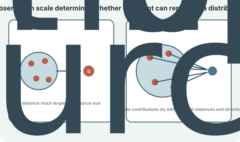
An extended object can be approximated as a point charge when observation distance is much larger than its size and distribution is sufficiently symmetric. Use total charge at an effective center. The approximation improves as size-to-distance ratio decreases. Near the object, distribution details matter. Sharp conductor features can create strong local fields.

For a continuous distribution, divide charge into elements $dq$. Each element produces $d\mathbf E=k\frac{dq}{r^2}\hat{\mathbf r}$. Integrate over the distribution. Symmetry can simplify the vector integral. Lines, surfaces, and volumes use corresponding charge densities.

Charge density symbols include linear $\lambda=\frac{dq}{d\ell}$, surface $\sigma=\frac{dq}{dA}$, and volume $\rho=\frac{dq}{dV}$. Their units are $\mathrm{\frac{C}{m}}$, $\mathrm{\frac{C}{m^2}}$, and $\mathrm{\frac{C}{m^3}}$. Context distinguishes volume charge density $\rho$ from mass density using definitions and units. Symbols are conventions, not meanings by themselves. The differential denominator identifies whether charge is distributed along length, area, or volume.

Electrostatic equilibrium in conductors

In an ideal conductor at electrostatic equilibrium, the electric field inside the conducting material is zero. Otherwise mobile charges would continue moving. Excess net charge lies on the surface. The conductor is an equipotential. The field just outside is perpendicular to the surface under ideal static conditions.

Charge density is not necessarily uniform over an irregular conductor. It becomes greater near regions of high curvature such as sharp points. Nearby external charges also redistribute surface charge. Treating all conductor charge as fixed at one center can fail. Boundary geometry matters.

Electrostatic shielding follows from conductor response. External fields rearrange surface charges so the field inside a closed conducting cavity can be zero when no internal charge is present under ideal conditions. A thin mesh can approximate shielding over wavelengths and openings suited to the problem. Real finite-frequency behavior adds complexity. Static conclusions should not be generalized without conditions.

Common mistakes and repairs

One mistake is inserting signed charges into a magnitude formula and accepting a negative force magnitude. Magnitude is nonnegative. Use absolute values for size and determine direction from attraction or repulsion. Alternatively, use a fully defined vector formula. Do not mix conventions mid-calculation.

Another mistake is adding force magnitudes from several charges. Draw each vector on the target. Resolve into components. Add signed components and reconstruct magnitude and direction. Symmetry can simplify only after directions are justified.

A third mistake is using centimetres or microcoulombs without conversion. Coulomb’s constant is stated in SI units. Convert distance to metres and charge to coulombs. Square the entire distance. Check that units reduce to newtons.

A reliable Coulomb-force workflow

First identify the target and all source charges. Draw positions with distances in metres. Mark charge signs and choose coordinate axes. Predict each force direction using attraction or repulsion. State whether point-charge and electrostatic approximations are reasonable.

Second calculate each magnitude with $F=k\frac{|q_iq_T|}{r_i^2}$. Attach the previously determined vector direction. Resolve into components. Add components to obtain net force. Use symmetry before arithmetic when applicable.

Third verify. Check inverse-square scaling and SI units. Confirm Newton’s third-law direction for a pair. Test limiting cases such as large distance or zero source charge. Explain what would change for an extended distribution, dielectric medium, or moving charge.

Retrieval practice and synthesis

Without looking back, state conservation and quantization of charge. Calculate the number of excess electrons corresponding to $-1.60\,\mathrm{nC}$. Include coulombs in the conversion. Explain why an initially neutral object can be attracted to a charged rod. Distinguish transfer from polarization.

Two charges $+4.00\,\mathrm{\mu C}$ and $-1.00\,\mathrm{\mu C}$ are $0.200\,\mathrm m$ apart. Calculate force magnitude and direction on each. Include $\mathrm{\frac{N\,m^2}{C^2}}$ in Coulomb’s constant. Explain why forces match while accelerations may not. Predict the magnitude if distance doubles.

Construct a three-charge line problem where two contributions cancel on a chosen target. Draw directions before choosing magnitudes. Write the equality needed for cancellation. Explain whether zero net force proves stable equilibrium. Identify one displacement direction that should be tested.